Diagnosing Overfitting in a PPI Transformer: Hyperparameter Search and What Actually Helped
Python
Deep Learning
Transformer
PyTorch
ESM2
Protein Language Models
Author
Jay Chung
Published
June 22, 2026
Summary
A hyperparameter search was conducted to diagnose and mitigate overfitting in a transformer-based model for predicting Protein-Protein Interactions (PPIs). The search explored variations in dropout rates, latent dimensions, and weight decay. The results showed that increasing dropout and reducing model size mildly improved generalization, while weight decay had a less pronounced effect. The best configuration achieved an AUROC improvement of ~0.02 on the leakage-reduced test set compared to the baseline. These results suggest that while hyperparameter tuning can provide modest gains, the model may have reached a possible performance ceiling given the current architecture and mean-pooled ESM2 embeddings. Further improvements are likely to require architectural changes or data augmentation strategies.
The problem
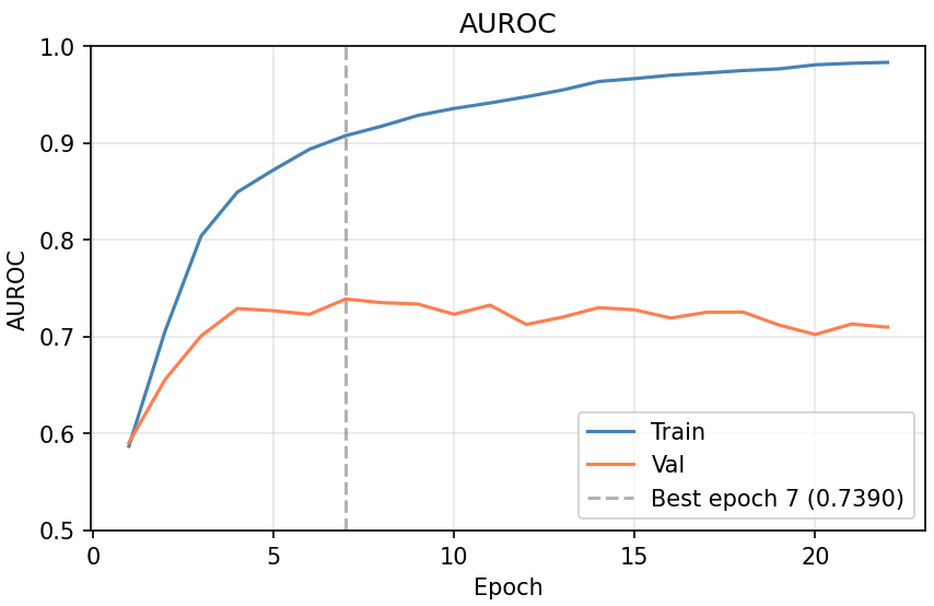
In my previous post, I built a transformer-based model to predict PPIs trained from the HuRI dataset. The model achieved an AUROC of 0.75 and accuracy of 0.67 on leakage-reduced test data, which is comparable to the performance of existing models in the literature (Reim et al. 2025). However, looking at the training and validation AUROC curves, it was clear that the model was overfitting to the training data quite early on. The training AUROC quickly reached 0.9 within the first few epochs, while the validation AUROC plateaued around 0.74 and even started to decline after epoch 10. This indicated that the model was learning patterns specific to the training data that did not generalize well to unseen data.
Training and validation AUROC curves showing overfitting.
Hypothesis
I hypothesized that the overfitting was due to the model being too complex for the amount of training data available, and that tuning the hyperparameters could help mitigate this issue. Specifically, I wanted to investigate how different hyperparameters such as latent dimension (model size), dropout rate, and weight decay affected the model’s performance and generalization ability.
Experimental design
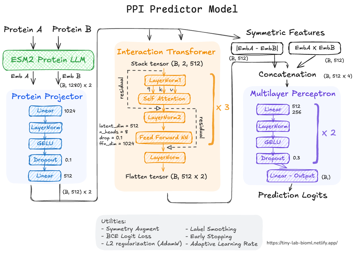
Let’s look at the model architecture again:
Model architecture diagram.
I defined 8 sets of hyperparameter configurations to test, including variations in dropout rates for the projection, attention, and MLP layers, as well as different latent dimensions and weight decay values. The configurations were designed to systematically explore the effects of increasing dropout, reducing model size, and applying stronger regularization through weight decay.
Here are some of the new functions that I defined for this hyperparameter search:
build_model_and_optimizer: This function takes in the hyperparameters and builds the PPIModel, sets up the optimizer with appropriate weight decay, and defines a learning rate scheduler. It also counts the number of trainable parameters in the model for later analysis.
run_hyperparameter_search: This function iterates through the defined CONFIGS, builds the model for each configuration, and runs the training loop. It records the training history, number of parameters, and checkpoint path for each configuration in a dictionary.
evaluate_all_on_test: After training all models, this function loads each model from its checkpoint and evaluates it on the test set, recording various metrics such as AUROC, AUPRC, F1 score, MCC, and accuracy in a DataFrame for easy comparison.
Code
# Function to instantiate model and utilitiesdef build_model_and_optimizer( proj_drop, attn_drop, mlp_drop, latent_dim, weight_decay, lr=1e-4,): torch.manual_seed(42) device = torch.device("cuda"if torch.cuda.is_available() else"cpu")print(f" Using device: {device}") model = PPIModel( esm2_dim =1280, latent_dim = latent_dim, num_heads =max(4, latent_dim //64), # scale heads with latent_dim num_layers =3, ffn_dim = latent_dim *2, hidden_dim = latent_dim //2, proj_drop = proj_drop, attn_drop = attn_drop, mlp_drop = mlp_drop, ).to(device) decay_params = [] no_decay_params = []for name, param in model.named_parameters():ifnot param.requires_grad:continueif'norm'in name or'bias'in name or param.dim() ==1: no_decay_params.append(param)else: decay_params.append(param) optimizer = torch.optim.AdamW([ {'params': decay_params, 'weight_decay': weight_decay}, {'params': no_decay_params, 'weight_decay': 0.0}, ], lr=1e-4) scheduler = torch.optim.lr_scheduler.ReduceLROnPlateau( optimizer, mode='max', patience=5, factor=0.5, min_lr=1e-7 ) n_params =sum(p.numel() for p in model.parameters() if p.requires_grad)return model, optimizer, scheduler, device, n_params
Code
# Function to run hp searchdef run_hyperparameter_search( configs = CONFIGS, train_loader =None, val_loader =None, loss_fn =None, save_path =None, n_epochs =100, early_stop_limit =15,):""" Iterate through CONFIGS to build model and perform training. Record metrics and hp information in a dictionary. """ all_results = {} # record: history, n_params, config, checkpointfor i, (label, dropout, latent_dim, weight_decay) inenumerate(configs): proj_drop, attn_drop, mlp_drop = dropoutprint(f"\n{'═'*65}")print(f" Config {i+1}/{len(configs)}: {label}")print(f" dropout=({proj_drop},{attn_drop},{mlp_drop}) "f"latent_dim={latent_dim} weight_decay={weight_decay}")print(f"{'═'*65}") model, optimizer, scheduler, device, n_params = build_model_and_optimizer( proj_drop, attn_drop, mlp_drop, latent_dim, weight_decay )print(f" Parameters: {n_params:,} ({n_params/len(train_loader.dataset):.1f} params/sample)") history = train( model = model, train_loader = train_loader, val_loader = val_loader, optimizer = optimizer, scheduler = scheduler, loss_fn = loss_fn, device = device, n_epochs = n_epochs, early_stop_limit = early_stop_limit, checkpoint_path =f"{save_path}/data/hparam_{label.replace('+','_')}.pt", ) all_results[label] = {"history": history,"n_params": n_params,"config": (dropout, latent_dim, weight_decay),"ckpt": f"{save_path}/data/hparam_{label.replace('+','_')}.pt", }print("All hyperparameter searches completed.")return all_results
Code
# Function to evaluate on test datadef evaluate_all_on_test(all_results, test_loader, loss_fn):""" Evaluate all models on test data. Build model -> load checkpoint -> evaluate -> record metrics. Return a pd.DataFrame with all metrics. """ device = torch.device("cuda"if torch.cuda.is_available() else"cpu") rows = []for label, res in all_results.items(): dropout, latent_dim, weight_decay = res["config"] proj_drop, attn_drop, mlp_drop = dropout model, _, _, _, n_params = build_model_and_optimizer( proj_drop, attn_drop, mlp_drop, latent_dim, weight_decay ) model.load_state_dict(torch.load(res["ckpt"])) model.to(device) model.eval() _, auroc, auprc, probs, labels = evaluate( model, test_loader, loss_fn, device ) preds = (probs >=0.5).astype(int) rows.append({"config": label,"n_params": n_params,"latent_dim": latent_dim,"dropout": f"({proj_drop},{attn_drop},{mlp_drop})","weight_decay": weight_decay,"test_auroc": round(auroc, 4),"test_auprc": round(auprc, 4),"f1": round(f1_score(labels, preds), 4),"precision": round(precision_score(labels, preds), 4),"recall": round(recall_score(labels, preds), 4),"mcc": round(matthews_corrcoef(labels, preds), 4),"accuracy": round(accuracy_score(labels, preds), 4),# Best val AUROC from training (for reference)"best_val_auroc": round(max(res["history"].history["val_auroc"]), 4),# Train-val gap at best epoch"gap_at_best": round( res["history"].history["train_auroc"][int(np.argmax(res["history"].history["val_auroc"])) ] -max(res["history"].history["val_auroc"]), 4 ), })print(f" {label:20s} test_auroc={auroc:.4f} test_auprc={auprc:.4f} "f"mcc={rows[-1]['mcc']:.4f}") df = pd.DataFrame(rows).sort_values("test_auroc", ascending=False).reset_index(drop=True)# columns are metrics, rows are configsreturn df
Results & discussions
The different hyperparameter configurations had varying effects on the training dynamics and final performance. To visualize these differences, I created several plotting functions:
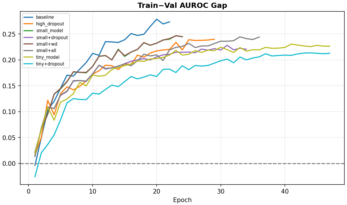
plot_learning_curves_comparison: This function plots the validation AUROC, AUPRC, validation loss, and the gap between training and validation AUROC for all configurations on the same axes. This allows for easy comparison of how each configuration affected the learning curves and overfitting behavior.
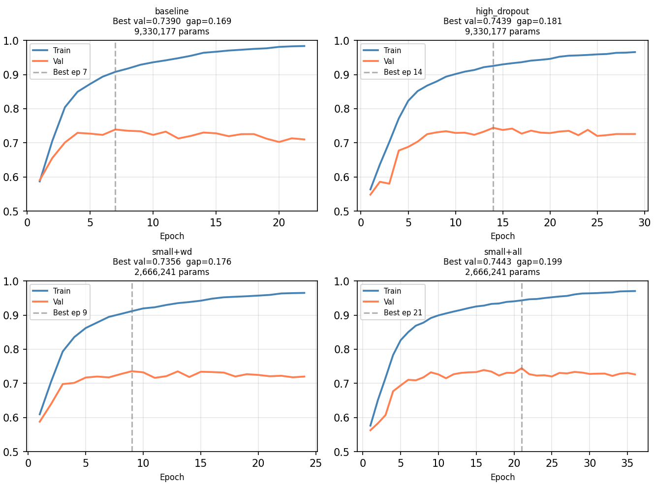
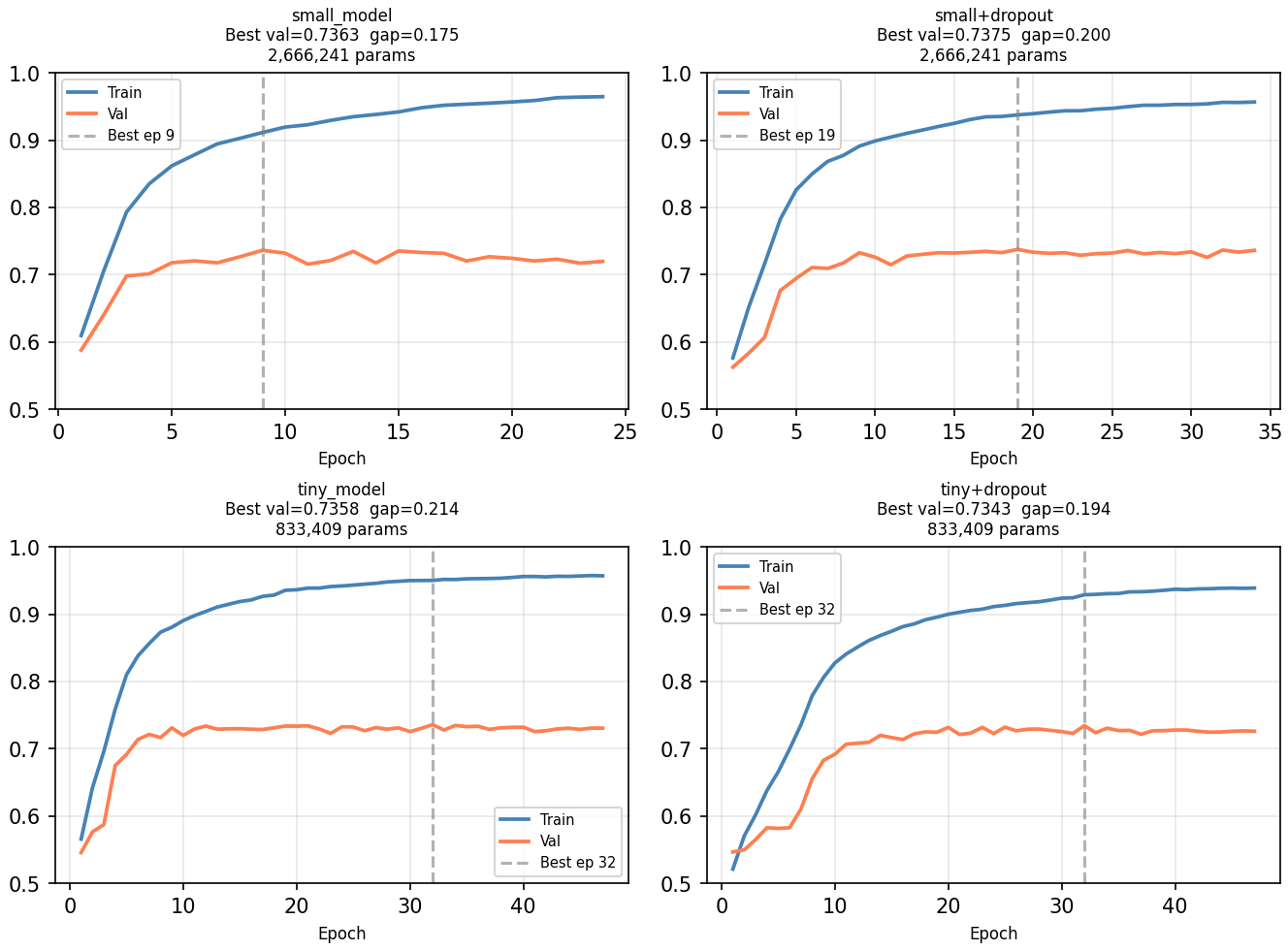
plot_train_val_curves_per_config: This function creates a grid of plots, where each plot shows the training and validation AUROC curves for a single configuration. This is a more traditional way to diagnose overfitting for each model individually.
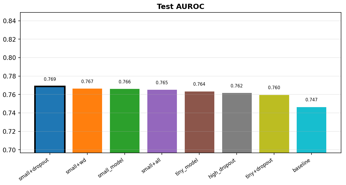
plot_test_metrics_comparison: This function creates bar charts comparing the test AUROC, AUPRC, F1 score, and MCC across all configurations. The bars are annotated with the metric values and the best-performing configuration is highlighted.
Code
def plot_learning_curves_comparison(all_results, save_path=None):""" Plots val AUROC, val AUPRC, val Loss, and train/val AUROC gap for all configs on the same axes for easy comparison. """ labels =list(all_results.keys()) colors = cm.tab10(np.linspace(0, 1, len(labels))) fig, axes = plt.subplots(2, 2, figsize=(16, 10)) fig.suptitle("Hyperparameter Comparison — Learning Curves", fontsize=14, fontweight='bold') metrics = [ ("val_auroc", axes[0, 0], "Val AUROC", "max", [0.5, 1.0]), ("val_auprc", axes[0, 1], "Val AUPRC", "max", [0.5, 1.0]), ("val_loss", axes[1, 0], "Val Loss", "min", None), (None, axes[1, 1], "Train−Val AUROC Gap", "min", None), # special ]for metric_key, ax, title, _, ylim in metrics:for label, color inzip(labels, colors): h = all_results[label]["history"].history epochs =range(1, len(h["train_auroc"]) +1)if metric_key isNone:# Gap plot gap = [tr - vl for tr, vl inzip(h["train_auroc"], h["val_auroc"])] ax.plot(epochs, gap, label=label, color=color, linewidth=1.8) ax.axhline(y=0, color='gray', linestyle='--', alpha=0.4)else: ax.plot(epochs, h[metric_key], label=label, color=color, linewidth=1.8)# Mark best val AUROC epoch with a dot best_ep =int(np.argmax(h["val_auroc"])) +1 best_val = h["val_auroc"][best_ep -1]if metric_key =="val_auroc": ax.scatter(best_ep, best_val, color=color, s=60, zorder=5) ax.set_title(title, fontweight='bold') ax.set_xlabel("Epoch") ax.grid(True, alpha=0.3)if ylim: ax.set_ylim(ylim) ax.legend(fontsize=7, loc='best') plt.tight_layout()if save_path: out =f"{save_path}/hparam_learning_curves.png" plt.savefig(out, dpi=150, bbox_inches='tight')print(f"Saved → {out}") plt.show()
Code
def plot_train_val_curves_per_config(all_results, save_path=None):""" For each config, plots train vs val AUROC side by side — the standard overfitting diagnostic view. """ n =len(all_results) ncols =4 nrows =int(np.ceil(n / ncols)) fig, axes = plt.subplots(nrows, ncols, figsize=(ncols *4.5, nrows *3.5)) axes = axes.flatten() fig.suptitle("Train vs Val AUROC per Config", fontsize=13, fontweight='bold')for i, (label, res) inenumerate(all_results.items()): h = res["history"].history ax = axes[i] eps =range(1, len(h["train_auroc"]) +1) best_ep =int(np.argmax(h["val_auroc"])) +1 ax.plot(eps, h["train_auroc"], label="Train", color="steelblue", lw=1.8) ax.plot(eps, h["val_auroc"], label="Val", color="coral", lw=1.8) ax.axvline(x=best_ep, color='gray', linestyle='--', alpha=0.6, label=f"Best ep {best_ep}") best_val =max(h["val_auroc"]) gap = h["train_auroc"][best_ep-1] - best_val n_params = res["n_params"] ax.set_title(f"{label}\nBest val={best_val:.4f} gap={gap:.3f}\n{n_params:,} params", fontsize=8) ax.set_ylim([0.5, 1.0]) ax.set_xlabel("Epoch", fontsize=8) ax.legend(fontsize=7) ax.grid(True, alpha=0.3)# Hide unused subplotsfor j inrange(i +1, len(axes)): axes[j].set_visible(False) plt.tight_layout()if save_path: out =f"{save_path}/hparam_per_config_curves.png" plt.savefig(out, dpi=150, bbox_inches='tight')print(f"Saved → {out}") plt.show()
Code
def plot_test_metrics_comparison(results_df, save_path=None):""" Bar chart comparing test AUROC, AUPRC, F1, and MCC across all configs. Configs sorted by test AUROC descending. """ metrics = ["test_auroc", "test_auprc", "f1", "mcc"] titles = ["Test AUROC", "Test AUPRC", "F1 Score", "MCC"] labels = results_df["config"].tolist() x = np.arange(len(labels)) colors = cm.tab10(np.linspace(0, 1, len(labels))) fig, axes = plt.subplots(2, 2, figsize=(16, 9)) fig.suptitle("Test Set Performance by Hyperparameter Config", fontsize=13, fontweight='bold')for ax, metric, title inzip(axes.flatten(), metrics, titles): vals = results_df[metric].tolist() bars = ax.bar(x, vals, color=colors, edgecolor='white', linewidth=0.5)# Annotate barsfor bar, v inzip(bars, vals): ax.text(bar.get_x() + bar.get_width() /2, bar.get_height() +0.005,f"{v:.3f}", ha='center', va='bottom', fontsize=7) ax.set_title(title, fontweight='bold') ax.set_xticks(x) ax.set_xticklabels(labels, rotation=35, ha='right', fontsize=8) ax.set_ylim([max(0, min(vals) -0.05), min(1.0, max(vals) +0.08)]) ax.grid(True, axis='y', alpha=0.3)# Highlight best best_idx =int(np.argmax(vals)) bars[best_idx].set_edgecolor('black') bars[best_idx].set_linewidth(2.5) plt.tight_layout()if save_path: out =f"{save_path}/hparam_test_metrics.png" plt.savefig(out, dpi=150, bbox_inches='tight')print(f"Saved → {out}") plt.show()
Now let’s run everything and discuss the results as we go along.
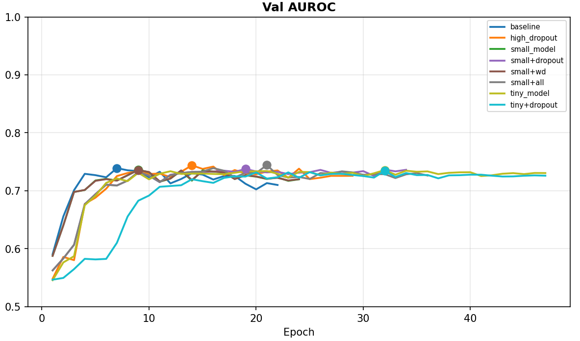
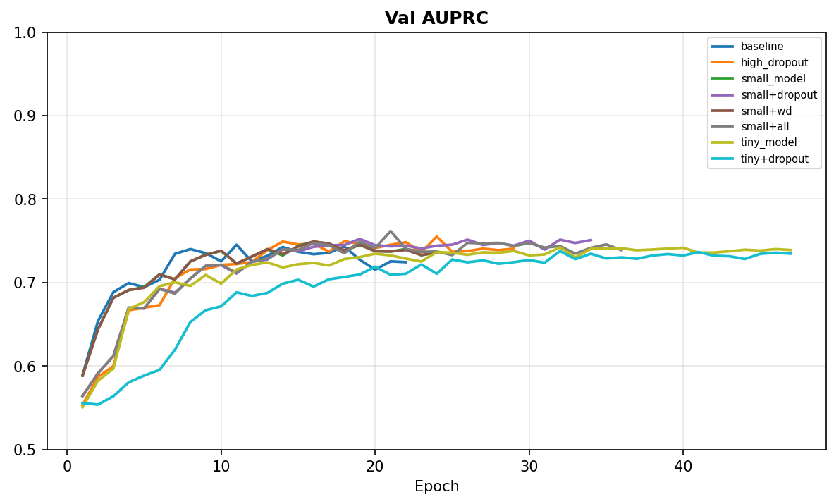
Looking at validation AUROC and AUPRC, the metrics appear to peak at around 0.74 no matter the model configuration, suggesting that this might be the performance plateau that the current data setting can reach - meaning that the bottleneck is likely not the model architecture, but the limitation of mean-pooled ESM2 embeddings and the size of the HuRI dataset to generalize to unseen PPIs.
Looking at the train-val AUROC gap curve, it appears that reducing the model size or increasing regularization/dropouts did reduce the severity of overfitting, albeit not sufficient to significantly improve the best validation AUROC.
Let’s look at the actual train vs val AUROC curves for each configuration to see how the overfitting dynamics differ:
Code
# Plot learning curves: compare train vs. val per configplot_train_val_curves_per_config(all_results, save_path=save_path)
Looking at the per-config train-vs-val curves, the reduction in the train-val gap is driven primarily by a lower training AUROC at later epochs — not by a meaningful increase in validation AUROC.
Now we will evaluate the best model checkpoint for each config on the leakage-reduced test set to see if there is any improvement in test performance:
# Plot test metrics across configsplot_test_metrics_comparison(results_df, save_path=save_path)
Test AUROC ranked by AUROC
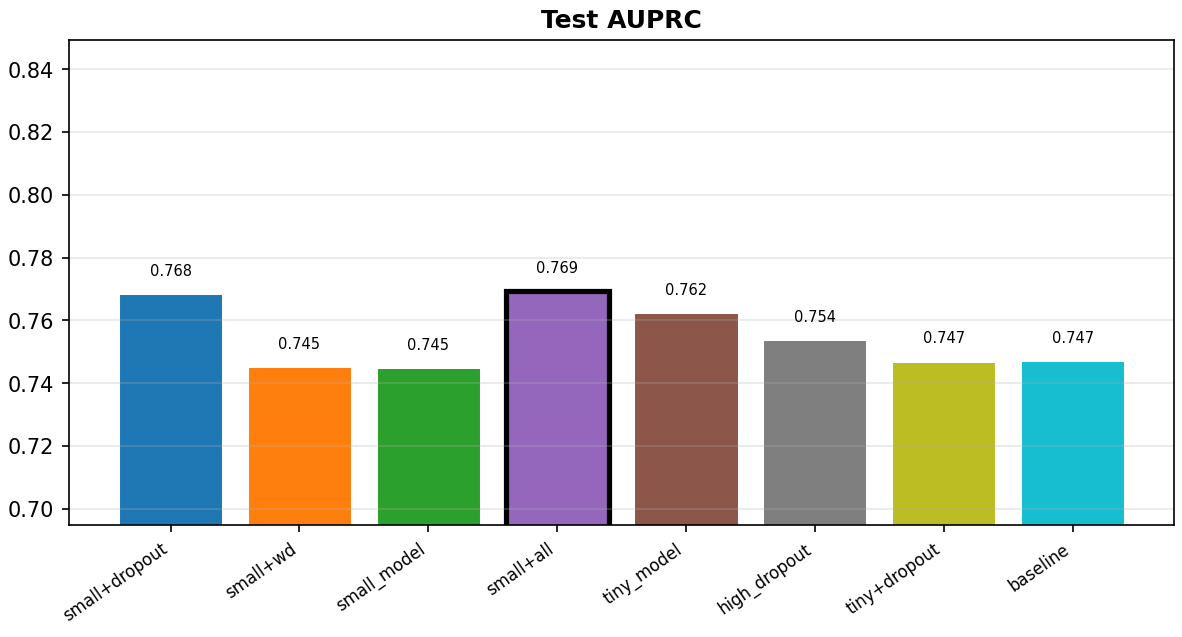
Test AUPRC ranked by AUROC
Looking at the test metrics, which is the most important indication of how the model is performing, the smaller models with stronger dropouts/regularization generally improved the performance when compared with the baseline. Among these models, the “small+dropout” showed consistently higher AUROC and AUPRC, which both improved by ~0.02, suggesting that this model config is most adequate for the data.
Why is there a disconnect between some AUROCs vs AUPRCs? AUROC measures the model’s ability to rank positives above negatives across all classification thresholds, treating both classes symmetrically. AUPRC, by contrast, focuses on the precision-recall trade-off and is more sensitive to how well the model identifies true positives with high confidence. Even on balanced datasets, the two metrics can diverge when a model ranks most positives correctly (good AUROC) but with poor confidence separation at high-score ranges (lower AUPRC). This is worth keeping in mind when calling out the best-performing model — a configuration that wins on AUROC may not win on AUPRC, as we see here with small+dropout vs small+all.
Future directions
Now that there is a better understanding of how hyperparameter tuning affects the performance of the PPI transformer model, perhaps there are other avenues to explore. In future posts, I’ll investigate whether per-token (non-mean-pooled) embeddings or isoform-based data augmentation — selecting multiple isoforms per protein within a defined similarity band — can push past this ceiling.
Disclosures
The code was written with the aid of Claude Sonnet 4.6, and the model training was performed on Google Colab Pro+ with a Tesla T4 GPU. The accuracy of the codes were verified by the author.