Code
from tdc.multi_pred import PPI

# Load the HuRI dataset
data = PPI(name='HuRI')
ppi_data = data.get_data()
print(ppi_data)Using the PyTorch framework, I built a transformer-based model to predict Protein-Protein Interactions (PPIs) trained from the HuRI dataset. The workflow takes a pair of protein sequences as input, extracts ESM2 embeddings, and predicts the probability of interaction. The model achieved an AUPRC of 0.75 and accuracy of 0.67 on leakage-reduced test data, which is comparable to the performance of existing models in the literature. The transformer model significantly outperformed a baseline random forest model, which achieved an AUPRC of 0.62 and accuracy of 0.59 on the same test set.
Why is it important to build a PPI predictor?
Drug discovery and disease mechanism: PPI is fundamental to how proteins carry out their functions in the cell. Identifying interaction partners of a drug target can help us understand the target’s biological role and its involvement in disease pathways. Many diseases involve dysregulated PPIs, often by disrupting normal interactions or creating new ones through functional mutations. Predicting how these mutations affect PPIs can help us better understand disease mechanisms and identify potential therapeutic targets. In addition, a PPI predictor model can be used for off-target screening of protein biologics, which is crucial for drug safety and efficacy.
Proteome-wide interaction networks: Current large-scale PPI screen like HuRI contains roughly ~9,000 proteins, while the human proteome contains ~20,000 proteins, many of which are understudied. A trained model can be used to explore these unknown PPIs, potentially expanding our knowledge of interactome without the costs and time of experimental screens. A generalized PPI prediction model can be applied to other species as well, or to cross-species interaction like virus-host protein interaction, helping us understand the biology of non-model organisms and infectious diseases.
Contributing to the PPI deep learning field: By utilizing state-of-the-art models like ESM2 and transformer architectures, I aim to see if building a model with comparable performance to existing models is possible. This contributes to the broader question of how much interaction-relevant information is already encoded in ESM2 embeddings, and whether further optimization of the model architecture can lead to significant performance gains. I will also address the issue of data leakage in PPI prediction, which is a common pitfall that can lead to overestimated performance. By carefully designing the training and evaluation strategy to avoid data leakage, I hope to provide a more realistic assessment of the model’s predictive power.
Last year, a paper by Reim et al. (2025) compared various deep learning architectures for PPI prediction, including models with attention mechanisms and incorporation of ESM2 protein language model. They found that regardless of the model architecture or the hyperparameter space, all models seemed to plateau at an accuracy of 0.65. They concluded that any performance gains observed are attributable to the use of ESM2 embeddings, rather than the model architecture itself. The paper also provided some interesting observations about the ESM2 model usage; for example, models profited from smaller embeddings (t33), and that per-token embeddings (sequence information preserved) did not yield better performance than per-protein embeddings (mean embeddings across sequence).
Inspired by this paper, I want to see if I can build a model with comparable performance, albeit with a different model design. I decided to use the HuRI PPI dataset for training and evaluation, rather than the HIPPIE dataset used in the paper. The HuRI dataset came from a Yeast-2-Hybrid (Y2H) screen that contains ~9,000 proteins and ~64,000 experimental validated interactions. The HIPPIE dataset is a literature-curated dataset that is much larger but may also bias toward more well-studied proteins. Due to the difference in dataset size and quality, my result may not be directly comparable to the Reim et al. paper, but I will compare the transformer performance with a baseline random forest model to see if the transformer architecture provides any performance gain over a simpler model.
Many papers in the PPI prediction field have pointed out the issue of data leakage, which is when the same or similar proteins appear in both training and test sets, leading to overestimated performance. To address this, I will implement a leakage-reduced splitting strategy that ensures that proteins in the test set are not similar or present in the training set. This will provide a more realistic assessment of the model’s generalization ability.
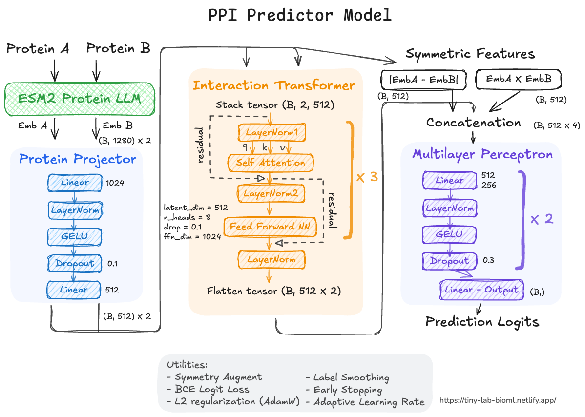
The model contains four main components:
t33_650M_UR50D variant of ESM2, which has been shown to perform well for PPI prediction in the Reim et al. paper.|EmbA - EmbB| and EmbA * EmbB (absolute difference and products), which gave the model more flexibility to learn the interaction-relevant information. The MLP will output a probability score indicating the likelihood of interaction between the two proteins.One caveat for the HuRI data is that the Y2H experiment is prone to false positives, which might exacerbate the issue of overfitting, meaning that the model will predict well on training data but could not generalized to unseen test data. To deal with this, these features were added to the model design:
Another consideration is the size of the model vs. training sample size. With around 50k of HuRI training samples, this is on the lower side of training a 9.3 million parameters transformer model. 9.3M params / 50k samples = 180 params per sample. Normally it would be great to get this ratio to < 100 to prevent overfitting, but given that the model is not learning everything from scratch - ESM2 did the initial heavy lifting - this setting might be acceptable.
First, I will download the positive interactions HuRI data from TDC, and then process and clean up the data. A protein similarity-aware split will be performed to obtain the train, validation and test data. HuRI data only contains positive interactions, so I will also perform negative sampling to generate negative interaction samples for each of the split. This is done after the splitting to avoid further data leakage, as the negative samples are generated based on the proteins present in each split.
from tdc.multi_pred import PPI
# Load the HuRI dataset
data = PPI(name='HuRI')
ppi_data = data.get_data()
print(ppi_data)Output:
           Protein1_ID                                           Protein1  \
0      ENSG00000000005  MAKNPPENCEDCHILNAEAFKSKKICKSLKICGLVFGILALTLIVL...
1      ENSG00000000005  MAKNPPENCEDCHILNAEAFKSKKICKSLKICGLVFGILALTLIVL...
2      ENSG00000000005  MAKNPPENCEDCHILNAEAFKSKKICKSLKICGLVFGILALTLIVL...
3      ENSG00000000005  MAKNPPENCEDCHILNAEAFKSKKICKSLKICGLVFGILALTLIVL...
4      ENSG00000000005  MAKNPPENCEDCHILNAEAFKSKKICKSLKICGLVFGILALTLIVL...
...                ...                                                ...
52364  ENSG00000273899  MGRNKKKKRDGDDRRPRLVLSFDEEKRREYLTGFHKRKVERKKAAI...
52365  ENSG00000275302  MKLCVTVLSLLMLVAAFCSPALSAPMGSDPPTACCFSYTARKLPRN...
52366  ENSG00000275774  MASNVTNKMDPHSVNSRVFIGNLNTLVVKKSDVEAIFSKYGKIAGC...
52367  ENSG00000276070  MKLCVTVLSLLVLVAAFCSLALSAPMGSDPPTACCFSYTARKLPRN...
52368  ENSG00000276076  MPVCPGDSHRPPKALPHLVCGRRGRQVRSDRDKFVIFLDVKHFSPE...

           Protein2_ID                                           Protein2  Y
0      ENSG00000061656  MRRSSRPGSASSSRKHTPNFFSENSSMSITSEDSKGLRSAEPGPGE...  1
1      ENSG00000099968  MASSSTVPLGFHYETKYVVLSYLGLLSQEKLQEQHLSSPQGVQLDI...  1
2      ENSG00000104765  MSSHLVEPPPPLHNNNNNCEENEQSLPPPAGLNSSWVELPMNSSNG...  1
3      ENSG00000105383  MPLLLLLPLLWAGALAMDPNFWLQVQESVTVQEGLCVLVPCTFFHP...  1
4      ENSG00000114455  MKAQTALSFFLILITSLSGSQGIFPLAFFIYVPMNEQIVIGRLDED...  1
...                ...                                                ... ..
52364  ENSG00000273899  MGRNKKKKRDGDDRRPRLVLSFDEEKRREYLTGFHKRKVERKKAAI...  1
52365  ENSG00000278619  MEVMDVFSTDDLTGFLQTKAQQGWLVAGTVGCPSTEDPQSSEIPIM...  1
52366  ENSG00000275774  MASNVTNKMDPHSVNSRVFIGNLNTLVVKKSDVEAIFSKYGKIAGC...  1
52367  ENSG00000278619  MEVMDVFSTDDLTGFLQTKAQQGWLVAGTVGCPSTEDPQSSEIPIM...  1
52368  ENSG00000276076  MPVCPGDSHRPPKALPHLVCGRRGRQVRSDRDKFVIFLDVKHFSPE...  1

[52369 rows x 5 columns]
There are 52,369 positive interactions in the HuRI dataset. The “Protein1_ID” and “Protein2_ID” columns contain the Ensembl gene IDs of the interacting proteins, while the “Protein1” and “Protein2” columns contain the corresponding amino acid sequences. The “Y” column indicates that these are positive interactions (Y=1).
In this dataset, some proteins have multiple sequences associated with them, which may represent different isoforms or variants. The sequences are separated by asterisks (*). For example, if a protein has two sequences, the “Protein1” column may contain “MSEQ1*MSEQ2”. To make sure I don’t exclude any sequence motifs, I will take the longest isoform for each gene name. This is a simplification, as negative samples may be confounded by the inclusion of interaction motifs that are actually not present in the experiment. But it is a necessary step to train the model. Here I will make a dictionary mapping each gene name to its longest isoform.
def create_protein_sequence_dict(df):
    protein_dict = {}
    for index, row in df.iterrows():
        protein1_id = row["Protein1_ID"]
        protein2_id = row["Protein2_ID"]
        protein1_seq = row["Protein1"]
        protein2_seq = row["Protein2"]
        if protein1_id not in protein_dict:
            protein_dict[protein1_id] = max(protein1_seq.split("*"), key=len)  # Take the longest sequence if there are multiple
        if protein2_id not in protein_dict:
            protein_dict[protein2_id] = max(protein2_seq.split("*"), key=len)
    return protein_dict

protein_sequence_dict = create_protein_sequence_dict(ppi_data)

# Save protein sequence dictionary locally
import numpy as np
save_path = "/path_to_data"
np.save(f"{save_path}/data/protein_sequence_dict.npy", protein_sequence_dict)# Sequence length statistics: max, min, mean, median
from statistics import median
sequence_lengths = [len(seq) for seq in protein_sequence_dict.values()]
print(f"Max protein sequence length: {max(sequence_lengths)}")
print(f"Min protein sequence length: {min(sequence_lengths)}")
print(f"Mean protein sequence length: {sum(sequence_lengths) / len(sequence_lengths):.0f}")
print(f"Median protein sequence length: {median(sequence_lengths)}")Output:
Max protein sequence length: 6907
Min protein sequence length: 25
Mean protein sequence length: 522
Median protein sequence length: 420.0# Plot the distribution of sequence lengths
# ESM2 has a maximum sequence length of 1022
import matplotlib.pyplot as plt
plt.hist(sequence_lengths, bins=50, color='blue', edgecolor='black')
plt.title('Distribution of Protein Sequence Lengths')
plt.xlabel('Sequence Length')
plt.ylabel('Frequency')
plt.axvline(x=1022, color='red', linestyle='--', label='ESM2 max length: 1022')
plt.legend()
plt.show()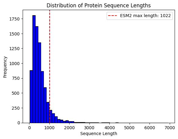
# Map cleaned protein dictionary to the PPI data
ppi_data["Protein1"] = ppi_data["Protein1_ID"].map(protein_sequence_dict)
ppi_data["Protein2"] = ppi_data["Protein2_ID"].map(protein_sequence_dict)

# Check that the sequences look fine
all_proteins = pd.unique(pd.concat([ppi_data['Protein1'], ppi_data['Protein2']]))

print(f"Total unique proteins: {len(all_proteins)}")
print(f"Empty sequences      : {(pd.Series(all_proteins).str.len() == 0).sum()}")
print(f"Contains '*'         : {pd.Series(all_proteins).str.contains('\\*').sum()}")
print(f"Contains whitespace  : {pd.Series(all_proteins).str.contains('\\s').sum()}")
print(f"Min length           : {pd.Series(all_proteins).str.len().min()}")
print(f"Max length           : {pd.Series(all_proteins).str.len().max()}")
Output:
Total unique proteins: 8170
Empty sequences      : 0
Contains '*'         : 0
Contains whitespace  : 0
Min length           : 25
Max length           : 6907
As we can see, some proteins are longer than what the ESM2 model can handle (max 1022 amino acids). To be on the conservative side, I will remove these proteins from the dataset.
# We have another problem now: some proteins are longer than 1022 amino acids, which is the maximum sequence length that ESM2 can handle.
def filter_long_proteins(df, protein_dict, max_length=1022):
    filtered_rows = []
    for index, row in df.iterrows():
        protein1_id = row["Protein1_ID"]
        protein2_id = row["Protein2_ID"]
        if len(protein_dict[protein1_id]) <= max_length and len(protein_dict[protein2_id]) <= max_length:
            filtered_rows.append(row)
    print(f"Removed {len(df) - len(filtered_rows)} protein pairs with sequences longer than {max_length} amino acids")
    print(f"\nRemaining protein pairs: {len(filtered_rows)}")
    return pd.DataFrame(filtered_rows)

ppi_data_filtered = filter_long_proteins(ppi_data, protein_sequence_dict)

# If two genes both map to the same sequence after picking longest, will get duplicate (Protein1, Protein2) pairs - remove these
before = len(ppi_data_filtered)
ppi_data_filtered = ppi_data_filtered.drop_duplicates(subset=['Protein1', 'Protein2'])
print(f"Removed {before - len(ppi_data_filtered)} duplicate pairs after isoform resolution")
Output:
Removed 7179 protein pairs with sequences longer than 1022 amino acids

Remaining protein pairs: 45190

Removed 689 duplicate pairs after isoform resolutiontotal_pairs = len(ppi_data_filtered)
total_proteins = len(set(ppi_data_filtered['Protein1'].tolist() + ppi_data_filtered['Protein2'].tolist()))
pos_perct = len(ppi_data_filtered[ppi_data_filtered['Y'] == 1]) / total_pairs
neg_perct = len(ppi_data_filtered[ppi_data_filtered['Y'] == 0]) / total_pairs
print(f"total protein pairs: {total_pairs} | total unique proteins: {total_proteins} | positive: {pos_perct:.1%} | negative: {neg_perct:.1%}")
# Save processed data locally
ppi_data_filtered.to_feather(f"{save_path}/data/ppi_data_filtered.feather")Output:
total protein pairs: 44501 | total unique proteins: 7357 | positive: 100.0% | negative: 0.0%I get 44,501 positive protein pairs after filtering out long sequences and resolving isoforms. There are 7,357 unique proteins in these pairs. The dataset is currently imbalanced with 100% positive samples, so I will need to perform negative sampling to generate negative interaction samples for training the model. I will do that after the train-val-test split to avoid data leakage.
Here I employed a similarity aware split with CD-HIT to ensure that proteins similar to the test set are not seen during training. This is a rigorous strategy that clusters proteins by sequence similarity before splitting, thus making sure that similar proteins do not show up across the train, validation and test set. A similarity split on HuRI data is estimated to result in ~40-50% of data loss.
def similarity_aware_split(
    df: pd.DataFrame,
    protein_col_a: str = 'Protein1',
    protein_col_b: str = 'Protein2',
    similarity_thr: float = 0.4,
    train_frac: float = 0.70,
    val_frac: float = 0.15,
    test_frac: float = 0.15,
    random_state: int = 42,
    verbose: bool = True,
) -> tuple[pd.DataFrame, pd.DataFrame, pd.DataFrame]:

    import subprocess, tempfile, os
    from Bio import SeqIO
    from Bio.SeqRecord import SeqRecord
    from Bio.Seq import Seq
    import numpy as np
    import pandas as pd

    # Guard against unsupported threshold
    if similarity_thr < 0.4:
        raise ValueError(
            f"CD-HIT requires similarity_thr >= 0.4. Got {similarity_thr}.\n"
            f"Use similarity_aware_split_nokmer() for thresholds below 0.4."
        )

    # Correct word size per CD-HIT documentation
    if   similarity_thr >= 0.7: word_size = 5
    elif similarity_thr >= 0.6: word_size = 4
    elif similarity_thr >= 0.5: word_size = 3
    else:                       word_size = 2

    all_proteins = pd.unique(
        pd.concat([df[protein_col_a], df[protein_col_b]])
    )
    seq_to_id = {seq: f"prot_{i}" for i, seq in enumerate(all_proteins)}
    id_to_seq = {v: k for k, v in seq_to_id.items()}

    if verbose:
        print(f"Running CD-HIT on {len(all_proteins)} proteins "
              f"(similarity threshold: {similarity_thr:.0%}, "
              f"word size: {word_size})...")

    with tempfile.TemporaryDirectory() as tmpdir:
        fasta_path = os.path.join(tmpdir, "proteins.fasta")
        output_path = os.path.join(tmpdir, "clustered")
        cluster_path = output_path + ".clstr"

        records = [
            SeqRecord(Seq(seq), id=seq_to_id[seq], description="")
            for seq in all_proteins
        ]
        with open(fasta_path, 'w') as f:
            SeqIO.write(records, f, "fasta")

        cmd = [
            "cd-hit",
            "-i", fasta_path,
            "-o", output_path,
            "-c", str(similarity_thr),
            "-n", str(word_size),
            "-T", "4",
            "-M", "4000",
            "-d", "0",
        ]
        result = subprocess.run(cmd, capture_output=True, text=True)

        if result.returncode != 0:
            raise RuntimeError(
                f"CD-HIT failed (return code {result.returncode}):\n"
                f"STDOUT: {result.stdout[:300]}\n"
                f"STDERR: {result.stderr[:300]}"
            )

        # Parse cluster file
        protein_to_cluster = {}
        current_cluster = None
        with open(cluster_path) as f:
            for line in f:
                line = line.strip()
                if line.startswith('>Cluster'):
                    current_cluster = int(line.split()[1])
                elif line:
                    prot_id = line.split('>')[1].split('...')[0]
                    protein_to_cluster[prot_id] = current_cluster

    seq_to_cluster = {
        seq: protein_to_cluster[seq_to_id[seq]]
        for seq in all_proteins
    }

    # Save protein_to_cluster and seq_to_cluster locally as dataframe
    protein_to_cluster_df = pd.DataFrame.from_dict(protein_to_cluster, orient='index', columns=['Cluster'])
    protein_to_cluster_df.index.name = 'Protein_ID'
    protein_to_cluster_df.reset_index(inplace=True)
    protein_to_cluster_df.to_feather(f"{save_path}/data/protein_to_cluster.feather")
    seq_to_cluster_df = pd.DataFrame.from_dict(seq_to_cluster, orient='index', columns=['Cluster'])
    seq_to_cluster_df.index.name = 'Protein_ID'
    seq_to_cluster_df.reset_index(inplace=True)
    seq_to_cluster_df.to_feather(f"{save_path}/data/seq_to_cluster.feather")

    all_clusters = list(set(seq_to_cluster.values()))
    n_clusters = len(all_clusters)

    if verbose:
        print(f"  {len(all_proteins)} proteins → {n_clusters} clusters")

    # Split at cluster level
    rng = np.random.default_rng(random_state)
    rng.shuffle(all_clusters)

    n_train = int(n_clusters * train_frac)
    n_val = int(n_clusters * val_frac)

    train_clusters = set(all_clusters[:n_train])
    val_clusters = set(all_clusters[n_train : n_train + n_val])
    test_clusters = set(all_clusters[n_train + n_val:])

    def assign_split(row):
        ca = seq_to_cluster[row[protein_col_a]]
        cb = seq_to_cluster[row[protein_col_b]]
        if ca in train_clusters and cb in train_clusters: return 'train'
        if ca in val_clusters   and cb in val_clusters:   return 'val'
        if ca in test_clusters  and cb in test_clusters:  return 'test'
        return 'discard'

    df = df.copy()
    df['_split'] = df.apply(assign_split, axis=1)

    train_df = df[df['_split'] == 'train'].drop(columns='_split').reset_index(drop=True)
    val_df = df[df['_split'] == 'val'].drop(columns='_split').reset_index(drop=True)
    test_df = df[df['_split'] == 'test'].drop(columns='_split').reset_index(drop=True)
    discarded = (df['_split'] == 'discard').sum()

    if verbose:
        print(f"\nPair split:")
        print(f"  Train pairs    : {len(train_df)}")
        print(f"  Val pairs      : {len(val_df)}")
        print(f"  Test pairs     : {len(test_df)}")
        print(f"  Discarded pairs: {discarded}")

    return train_df, val_df, test_df

train_df, val_df, test_df = similarity_aware_split(ppi_data, similarity_thr=0.4)
Output:
Running CD-HIT on 7357 proteins (similarity threshold: 40%, word size: 2)...
  7357 proteins → 5967 clusters

Pair split:
  Train pairs    : 23653
  Val pairs      : 916
  Test pairs     : 903
  Discarded pairs: 19029
A total of 19,029 pairs were discarded because they contained proteins that were similar across splits. This is a significant reduction in data size, but it is necessary to ensure that the model’s performance is not overestimated due to data leakage.
Let’s verify that there is no protein overlap between the splits:
# A function to validate that no data leakage detected
def verify_no_leakage(
    train_df: pd.DataFrame,
    val_df: pd.DataFrame,
    test_df: pd.DataFrame,
    protein_col_a: str = 'Protein1',
    protein_col_b: str = 'Protein2',
) -> bool:
    """
    Asserts that no protein sequence appears in more than one split.
    Raises AssertionError if leakage is detected.
    """
    def get_proteins(df):
        return set(df[protein_col_a].tolist() + df[protein_col_b].tolist())

    train_proteins = get_proteins(train_df)
    val_proteins   = get_proteins(val_df)
    test_proteins  = get_proteins(test_df)

    train_val_overlap  = train_proteins & val_proteins
    train_test_overlap = train_proteins & test_proteins
    val_test_overlap   = val_proteins   & test_proteins

    print("\n── Leakage Verification ──────────────────────────")
    print(f"  Train proteins      : {len(train_proteins)}")
    print(f"  Val proteins        : {len(val_proteins)}")
    print(f"  Test proteins       : {len(test_proteins)}")
    print(f"  Train ∩ Val overlap : {len(train_val_overlap)}")
    print(f"  Train ∩ Test overlap: {len(train_test_overlap)}")
    print(f"  Val ∩ Test overlap  : {len(val_test_overlap)}")

    assert len(train_val_overlap)  == 0, \
        f"LEAKAGE: {len(train_val_overlap)} proteins in both train and val!"
    assert len(train_test_overlap) == 0, \
        f"LEAKAGE: {len(train_test_overlap)} proteins in both train and test!"
    assert len(val_test_overlap)   == 0, \
        f"LEAKAGE: {len(val_test_overlap)} proteins in both val and test!"

    print("  ✓ Zero protein overlap across all splits — no leakage detected")

verify_no_leakage(train_df, val_df, test_df)
Output:
── Leakage Verification ──────────────────────────
  Train proteins      : 4763
  Val proteins        : 549
  Test proteins       : 536
  Train ∩ Val overlap : 0
  Train ∩ Test overlap: 0
  Val ∩ Test overlap  : 0
✓ Zero protein overlap across all splits — no leakage detectedA helper function to sample negative pairs within each split:
import pandas as pd
import numpy as np
from itertools import combinations

def sample_negatives_within_split(
    pos_df: pd.DataFrame,
    protein_col_a: str = 'Protein1_ID',
    protein_col_b: str = 'Protein2_ID',
    frac: float = 1.0,
    random_state: int = 42,
    label_col: str = 'Y',
) -> pd.DataFrame:
    """
    Sample negative PPI pairs using ONLY proteins present in the given split.
    """

    # Make sure the df is all positives
    assert all(pos_df[label_col] == 1), "Input dataframe contains negative samples"

    rng = np.random.default_rng(random_state)

    # All proteins present in this split
    proteins = list(set(
        pos_df[protein_col_a].tolist() +
        pos_df[protein_col_b].tolist()
    ))

    # Build a set of known positives (both orderings) for fast lookup
    pos_set = set()
    for _, row in pos_df.iterrows():
        a, b = row[protein_col_a], row[protein_col_b]
        pos_set.add((a, b))
        pos_set.add((b, a))  # treat as symmetric

    n_negatives = int(len(pos_df) * frac)

    # Sample candidate negative pairs
    neg_pairs = []
    max_attempts = n_negatives * 20  # safety cap to avoid infinite loop
    attempts = 0

    while len(neg_pairs) < n_negatives and attempts < max_attempts:
        # Sample two different proteins at random
        a, b = rng.choice(proteins, size=2, replace=False)

        # Skip self-interactions and known positives
        if a == b:
            continue
        if (a, b) in pos_set:
            attempts += 1
            continue

        neg_pairs.append({protein_col_a: a, protein_col_b: b, label_col: 0})
        pos_set.add((a, b))   # prevent duplicate negatives
        pos_set.add((b, a))

        attempts += 1

    if len(neg_pairs) < n_negatives:
        print(f"Warning: only sampled {len(neg_pairs)}/{n_negatives} negatives "
              f"(protein pool may be too small for requested frac={frac})")

    neg_df = pd.DataFrame(neg_pairs)

    # Carry over other columns from pos_df (Protein1, Protein2 sequences etc.)
    # by joining on the ID columns if needed
    if 'Protein1' in pos_df.columns:
        seq_map = dict(zip(
            pos_df[protein_col_a].tolist() + pos_df[protein_col_b].tolist(),
            pos_df['Protein1'].tolist()    + pos_df['Protein2'].tolist()
        ))
        neg_df['Protein1'] = neg_df[protein_col_a].map(seq_map)
        neg_df['Protein2'] = neg_df[protein_col_b].map(seq_map)

    # Combine and shuffle
    combined = pd.concat(
        [pos_df.assign(**{label_col: 1}), neg_df],
        ignore_index=True
    ).sample(frac=1, random_state=random_state).reset_index(drop=True)

return combinedtrain_df = sample_negatives_within_split(train_df, frac=1.0, random_state=42)
val_df = sample_negatives_within_split(val_df, frac=1.0, random_state=43)
test_df = sample_negatives_within_split(test_df, frac=1.0, random_state=44)
# Check to make sure that positive and negative samples are balanced in all sets
for df, name in zip([train_df, val_df, test_df], ["training", "validation", "test"]):
positive_samples = df[df["Y"] == 1]
negative_samples = df[df["Y"] == 0]
print(f"Positive samples in {name} set: {len(positive_samples)}, Negative samples in {name} set: {len(negative_samples)}")Output:
Positive samples in training set: 23653, Negative samples in training set: 23653
Positive samples in validation set: 916, Negative samples in validation set: 916
Positive samples in test set: 903, Negative samples in test set: 903I will now extract ESM2 embeddings from protein sequences:
# Load sequence dictionary
import numpy as np
from transformers import AutoTokenizer, EsmModel
import torch
import math
from tqdm import tqdm

protein_sequence_dict = np.load(f"{save_path}/data/protein_sequence_dict.npy", allow_pickle='TRUE').item()

# Load pre-trained ESM2 model and tokenizer
model_checkpoint = "facebook/esm2_t33_650M_UR50D" # 1280 dim
tokenizer = AutoTokenizer.from_pretrained(model_checkpoint)
model = EsmModel.from_pretrained(model_checkpoint)
A helper function to extract ESM2 mean embeddings:
# Function to extract mean ESM2 embeddings
def extract_mean_embedding(
    sequence_dict : dict[str, str],
    tokenizer     : AutoTokenizer,
    model         : EsmModel,
    device        : torch.device | None = None,
    batch_size    : int = 64,
    max_len       : int = 1022,
) -> dict[str, np.ndarray]:

    """
    Extract ESM2 last hidden layer embeddings for protein sequences.
    Truncate sequences to max_len allowed for ESM2 input.
    Remove special tokens that are not amino acids.
    For each input protein, calculate mean embeddings across amino acids.
    """
    if device is None:
        device = torch.device("cuda" if torch.cuda.is_available() else "cpu")

    model = model.to(device)
    model.eval()

    sequence = list(sequence_dict.values())
    protein  = list(sequence_dict.keys())

    # Sort by length before batching to minimize padding waste
    paired   = sorted(zip(sequence, protein), key=lambda x: len(x[0]), reverse=True)
    sequence, protein = zip(*paired) # unzip
    sequence = list(sequence)
    protein  = list(protein)

    n_batches = math.ceil(len(sequence) / batch_size)
    all_batch_embeddings = []

    steps = tqdm(range(n_batches))
    for i in steps:
        steps.set_description(f"Processing batch {i+1}/{n_batches}")
        start = i * batch_size
        end   = (i + 1) * batch_size
        batch = sequence[start:end]

        # Tokenize with padding and max length
        inputs = tokenizer(
            batch,
            return_tensors = "pt",
            padding        = True,
            truncation     = True, # longer than max_len will be truncated
            max_length     = max_len,
        )
        inputs = {name: tensor.to(device) for name, tensor in inputs.items()}

        with torch.no_grad():
            outputs     = model(**inputs)
            hidden      = outputs.last_hidden_state      # (B, seq_len, 1280)
            attn_mask   = inputs['attention_mask']       # (B, seq_len)
            # 1: real token (including <cls> and <eos>), 0: padding token

            # Exclude <cls> (before start) and <eos> (end-of-sequence) from mean pool
            token_mask          = attn_mask.clone()
            token_mask[:, 0]    = 0                      # remove <cls>
            eos_positions       = attn_mask.sum(dim=1) - 1
            for b, eos_pos in enumerate(eos_positions):
                token_mask[b, eos_pos] = 0               # remove <eos>

            mask_expanded = token_mask.unsqueeze(-1).float() # (B, seq_len, 1)
            sum_emb       = (hidden * mask_expanded).sum(dim=1) # sum across seq_len
            n_tokens      = token_mask.sum(dim=1, keepdim=True).float()
            mean_emb      = (sum_emb / n_tokens).detach().cpu().numpy()

        all_batch_embeddings.append(mean_emb) # list of (B, 1280)

    embeddings = np.concatenate(all_batch_embeddings, axis=0) # stack along row: (all_prot, 1280)

    # Return as dictionary {protein_id: embedding_vector}
    embedding_dict = {prot: emb for prot, emb in zip(protein, embeddings)}
    return embedding_dict

# Extracting embeddings
embedding_dict = extract_mean_embedding(protein_sequence_dict, tokenizer, model)

# Convert to torch tensor dict and save
embedding_tensor_dict = {
    prot: torch.tensor(emb, dtype=torch.float32)
    for prot, emb in embedding_dict.items()
}
torch.save(embedding_tensor_dict, f"{save_path}/data/esm2_t33_650M_UR50D_embeddings_all_proteins_for_ppi.pt")
Output:
Processing batch 129/129: 100%|██████████| 129/129 [30:16<00:00, 14.08s/it]Let’s plot a t-SNE plot of the extracted ESM2 embeddings to see if there are any visible clusters:
# Get protein embedding dataframe with dataset split information
embedding_df = pd.DataFrame.from_dict(embedding_dict, orient='index')
embedding_df.index.name = 'Protein_ID'
embedding_df.reset_index(inplace=True)

train_prot = set(train_df['Protein1_ID'].tolist() + train_df['Protein2_ID'].tolist())
valid_prot = set(valid_df['Protein1_ID'].tolist() + valid_df['Protein2_ID'].tolist())
test_prot  = set(test_df['Protein1_ID'].tolist() + test_df['Protein2_ID'].tolist())

assign_split = lambda x: 'train' if x in train_prot else 'val' if x in valid_prot else 'test'
embedding_df['Split'] = embedding_df['Protein_ID'].apply(assign_split)

# Plot t-SNE scatter plot from the protein embeddings df colored by dataset split type
import matplotlib.pyplot as plt
import seaborn as sns
from sklearn.manifold import TSNE

tsne = TSNE(n_components=2, random_state=42).fit_transform(embedding_df.iloc[:, 1:-1])
tsne_df = pd.DataFrame(tsne, columns=['tsne1', 'tsne2'])
tsne_df["Split"] = embedding_df["Split"]

plt.figure(figsize=(10, 8))
sns.scatterplot(data=tsne_df, x='tsne1', y='tsne2', hue='Split', palette='Set2',
                alpha=0.7)
plt.title('t-SNE Visualization of Protein Embeddings')
plt.xlabel('t-SNE Dimension 1')
plt.ylabel('t-SNE Dimension 2')
plt.show()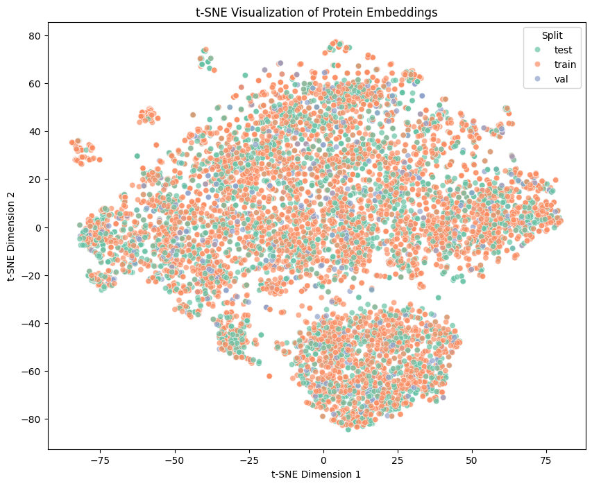
We can see that from the t-SNE representation of ESM2 embeddings, there are a few major and smaller clusters, likely representing proteins of different properties (e.g. structural, biochemical, sequence properties). Most proteins reside in larger clusters, and it is difficult to differentiate them with mean embeddings and a simple out-of-the-box t-SNE. Hopefully there are subtle information encoded within the embeddings that could be learned by the transformer model below.
Using PyTorch’s Dataset and DataLoader for data loading, shuffling and batching:
__getitem__. This saves RAM significantly by not repeated saving the same protein embedding in the dataset (e.g. some hub proteins like P53 might have many interactions and will appear many times in the PPI dataset).from torch.utils.data import Dataset, DataLoader
class PPIDataset(Dataset):
def __init__(
self,
df: pd.DataFrame,
embedding_dict: dict[str, torch.Tensor],
protein_a_id: str = 'Protein1_ID',
protein_b_id: str = 'Protein2_ID',
label_col: str = 'Y',
):
self.embedding_dict = embedding_dict
self.label_col = label_col
# Filter out rows where either protein has no embedding
# (e.g. proteins that failed extraction or were filtered)
mask = (
df[protein_a_id].isin(embedding_dict) &
df[protein_b_id].isin(embedding_dict)
)
n_dropped = (~mask).sum()
if n_dropped > 0:
print(f"Warning: dropped {n_dropped} pairs with missing embeddings")
df = df[mask].reset_index(drop=True)
# Store only the protein IDs and labels — not the embeddings themselves
# Embeddings are looked up at __getitem__ time from the shared dict
self.protein_a = df[protein_a_id].tolist()
self.protein_b = df[protein_b_id].tolist()
self.labels = torch.tensor(df[label_col].values, dtype=torch.float32)
def __len__(self) -> int:
return len(self.labels)
def __getitem__(self, idx: int) -> tuple[torch.Tensor, torch.Tensor, torch.Tensor]:
emb_a = self.embedding_dict[self.protein_a[idx]] # (1280,)
emb_b = self.embedding_dict[self.protein_b[idx]] # (1280,)
label = self.labels[idx] # model output is (B,) so this is ok
return emb_a, emb_b, label
# Build datasets for each split
train_dataset = PPIDataset(train_df, embedding_dict)
val_dataset = PPIDataset(valid_df, embedding_dict)
test_dataset = PPIDataset(test_df, embedding_dict)
# Build DataLoaders
train_loader = DataLoader(
train_dataset,
batch_size = 512,
shuffle = True, # shuffle every epoch during training
num_workers = 2, # parallel data loading
pin_memory = True, # faster CPU→GPU transfer
)
val_loader = DataLoader(
val_dataset,
batch_size = 512,
shuffle = False, # no need to shuffle val/test
num_workers = 2,
pin_memory = True,
)
test_loader = DataLoader(
test_dataset,
batch_size = 512,
shuffle = False,
num_workers = 2,
pin_memory = True,
)
# Verify shapes
emb_a, emb_b, labels = next(iter(train_loader))
print(emb_a.shape)
print(emb_b.shape)
print(labels.shape) Output:
torch.Size([512, 1280])
torch.Size([512, 1280])
torch.Size([512])Now I start building the model architecture. The model consists of three main components: ProteinProjector, InteractionTransformer, and PPIClassifier. I will build individual modules for each component, and then combine them into a full model.
import torch
import torch.nn as nn
import torch.nn.functional as F
import math

class ProteinProjector(nn.Module):
    """
    Projects a mean-pooled ESM2 embedding into a shared latent space.
    Both proteins pass through the same projector (shared weights).
    """
    def __init__(self, esm2_dim: int = 1280, latent_dim: int = 512, dropout: float = 0.1):
        super().__init__()
        self.net = nn.Sequential(
            nn.Linear(esm2_dim, latent_dim * 2),
            nn.LayerNorm(latent_dim * 2),
            nn.GELU(),
            nn.Dropout(dropout),
            nn.Linear(latent_dim * 2, latent_dim),
        )

    def forward(self, x: torch.Tensor) -> torch.Tensor:
return self.net(x)class InteractionTransformerLayer(nn.Module):
"""
Single transformer layer operating on a pair (2-token sequence).
"""
def __init__(self, latent_dim: int, num_heads: int, ffn_dim: int, dropout: float = 0.1):
super().__init__()
assert latent_dim % num_heads == 0, "latent_dim must be divisible by num_heads"
self.norm1 = nn.LayerNorm(latent_dim)
self.attn = nn.MultiheadAttention(
embed_dim = latent_dim,
num_heads = num_heads,
dropout = dropout,
batch_first = True, # (B, seq, dim) convention; defalut: (seq, B, dim)
)
self.norm2 = nn.LayerNorm(latent_dim)
self.ffn = nn.Sequential(
nn.Linear(latent_dim, ffn_dim),
nn.GELU(),
nn.Dropout(dropout),
nn.Linear(ffn_dim, latent_dim),
nn.Dropout(dropout),
)
def forward(self, x: torch.Tensor) -> torch.Tensor:
# Self-attention with pre-norm (each token attends to both tokens)
x_norm = self.norm1(x)
attn_out, _ = self.attn(x_norm, x_norm, x_norm) # attn_weight: (B, num_heads, 2, 2)
x = x + attn_out
# Feed-forward with pre-norm
x = x + self.ffn(self.norm2(x))
return xclass InteractionTransformer(nn.Module):
"""
Stack of InteractionTransformerLayers operating on the 2-token pair.
"""
def __init__(
self,
latent_dim: int = 512,
num_heads: int = 8,
num_layers: int = 3,
ffn_dim: int = 1024,
dropout: float = 0.1,
):
super().__init__()
self.layers = nn.ModuleList([
InteractionTransformerLayer(latent_dim, num_heads, ffn_dim, dropout)
for _ in range(num_layers)
]) # ModuleList is iterable at forward
self.norm = nn.LayerNorm(latent_dim) # final layer norm
def forward(self, emb_a: torch.Tensor, emb_b: torch.Tensor) -> torch.Tensor:
# Stack into a 2-token sequence: (B, 2, latent_dim)
x = torch.stack([emb_a, emb_b], dim=1) # stack at 1 position of shape
# this is because attention layer takes: (B, seq, dim)
for layer in self.layers:
x = layer(x)
x = self.norm(x) # (B, 2, latent_dim)
# Flatten the 2-token output into a single vector
# Shape: (B, latent_dim * 2)
fused = x.reshape(x.size(0), -1)
return fusedclass PPIClassifier(nn.Module):
"""
MLP head that takes the fused transformer output + symmetric features
and predicts PPI probability.
"""
def __init__(self, latent_dim: int = 512, hidden_dim: int = 256, dropout: float = 0.3):
super().__init__()
input_dim = latent_dim * 4 # transformer(2×latent) + symmetric(2×latent)
self.mlp = nn.Sequential(
nn.Linear(input_dim, hidden_dim * 2),
nn.LayerNorm(hidden_dim * 2),
nn.GELU(),
nn.Dropout(dropout),
nn.Linear(hidden_dim * 2, hidden_dim),
nn.LayerNorm(hidden_dim),
nn.GELU(),
nn.Dropout(dropout),
nn.Linear(hidden_dim, 1),
)
def forward(
self,
transformer_out: torch.Tensor, # (B, latent_dim * 2)
emb_a: torch.Tensor, # (B, latent_dim) — post-projection
emb_b: torch.Tensor, # (B, latent_dim)
) -> torch.Tensor:
# Symmetric features: invariant to A↔B swap
diff = torch.abs(emb_a - emb_b) # (B, latent_dim)
product = emb_a * emb_b # (B, latent_dim)
# Concatenate all signals
combined = torch.cat([transformer_out, diff, product], dim=-1) # (B, latent_dim*4)
logits = self.mlp(combined).squeeze(-1) # (B,)
return logitsNow we can combine all the components into a full PPI prediction model:
class PPIModel(nn.Module):
    """
    Full PPI prediction model.
    """
    def __init__(
        self,
        esm2_dim: int = 1280,
        latent_dim: int = 512,
        num_heads: int = 8,
        num_layers: int = 3,
        ffn_dim: int = 1024,
        hidden_dim: int = 256,
        proj_drop: float = 0.1,
        attn_drop: float = 0.1,
        mlp_drop: float = 0.3,
    ):
        super().__init__()

        self.projector = ProteinProjector(
            esm2_dim = esm2_dim,
            latent_dim = latent_dim,
            dropout = proj_drop,
        )
        self.transformer = InteractionTransformer(
            latent_dim = latent_dim,
            num_heads = num_heads,
            num_layers = num_layers,
            ffn_dim = ffn_dim,
            dropout = attn_drop,
        )
        self.classifier = PPIClassifier(
            latent_dim = latent_dim,
            hidden_dim = hidden_dim,
            dropout = mlp_drop,
        )

        self._init_weights()

    def _init_weights(self):
        """Xavier uniform (Glorot) for linear layers - better to stabilize gradient in deeper NN."""
        for module in self.modules():
            if isinstance(module, nn.Linear):
                nn.init.xavier_uniform_(module.weight)
                if module.bias is not None:
                    nn.init.zeros_(module.bias)

    def forward(
        self,
        emb_a: torch.Tensor,
        emb_b: torch.Tensor,
    ) -> torch.Tensor:
        # 1. Project both proteins into shared latent space (shared weights)
        proj_a = self.projector(emb_a)   # (B, latent_dim)
        proj_b = self.projector(emb_b)   # (B, latent_dim)

        # 2. Interaction transformer over the 2-token pair
        fused = self.transformer(proj_a, proj_b)   # (B, latent_dim * 2)

        # 3. MLP classifier with symmetric features
        logits = self.classifier(fused, proj_a, proj_b)   # (B,)
        return logits

    @torch.no_grad()
    def predict_proba(self, emb_a: torch.Tensor, emb_b: torch.Tensor) -> torch.Tensor:
        """Convenience method: returns interaction probability in [0, 1]."""
return torch.sigmoid(self.forward(emb_a, emb_b))Now I’ll define the loss function and a data augmentation function that randomly swaps the order of the protein pairs during training to enforce symmetry:
def get_loss_fn(label_smoothing: float = 0.05, pos_weight: float = None):
    """
    Returns BCEWithLogitsLoss with optional label smoothing and class weighting.
    """
    pw = torch.tensor([pos_weight]) if pos_weight is not None else None

    def loss_fn(logits: torch.Tensor, labels: torch.Tensor) -> torch.Tensor:
        if label_smoothing > 0:
            labels = labels * (1 - label_smoothing) + 0.5 * label_smoothing
        return nn.BCEWithLogitsLoss(pos_weight=pw)(logits, labels.float())

    return loss_fn

def symmetry_augment(emb_a: torch.Tensor,
                     emb_b: torch.Tensor,
                     labels: torch.Tensor):
    """
    Data augmentation: randomly swap A and B within a batch.
    PPI is symmetric, so (A,B) and (B,A) should predict the same label.
    Call this during training before passing to the model.
    """
    swap_mask = torch.rand(emb_a.size(0), device=emb_a.device) > 0.5
    emb_a_aug = torch.where(swap_mask.unsqueeze(1), emb_b, emb_a)
    emb_b_aug = torch.where(swap_mask.unsqueeze(1), emb_a, emb_b)
    return emb_a_aug, emb_b_aug, labels   # labels unchanged (symmetric)
How many parameters does the model have?
# Count parameters
total_params = sum(p.numel() for p in model.parameters())
print(f"Model parameters: {total_params:,}  ({total_params/1e6:.2f}M)")
Output:
Model parameters: 9,330,177 (9.33M)Instantiate the model, define the optimizer, scheduler, and loss function, and then run the training loop with validation at the end of each epoch.
torch.manual_seed(42)
device = torch.device("cuda" if torch.cuda.is_available() else "cpu")
print(f"Using device: {device}")

model = PPIModel(
    esm2_dim = 1280,
    latent_dim = 512,
    num_heads = 8,
    num_layers = 3,
    ffn_dim = 1024,
    hidden_dim = 256,
    proj_drop = 0.1,
    attn_drop = 0.1,
    mlp_drop = 0.3,
).to(device)

print(model)
Output:
Using device: cuda
PPIModel(
  (projector): ProteinProjector(
    (net): Sequential(
      (0): Linear(in_features=1280, out_features=1024, bias=True)
      (1): LayerNorm((1024,), eps=1e-05, elementwise_affine=True)
      (2): GELU(approximate='none')
      (3): Dropout(p=0.1, inplace=False)
      (4): Linear(in_features=1024, out_features=512, bias=True)
    )
  )
  (transformer): InteractionTransformer(
    (layers): ModuleList(
      (0-2): 3 x InteractionTransformerLayer(
        (norm1): LayerNorm((512,), eps=1e-05, elementwise_affine=True)
        (attn): MultiheadAttention(
          (out_proj): NonDynamicallyQuantizableLinear(in_features=512, out_features=512, bias=True)
        )
        (norm2): LayerNorm((512,), eps=1e-05, elementwise_affine=True)
        (ffn): Sequential(
          (0): Linear(in_features=512, out_features=1024, bias=True)
          (1): GELU(approximate='none')
          (2): Dropout(p=0.1, inplace=False)
          (3): Linear(in_features=1024, out_features=512, bias=True)
          (4): Dropout(p=0.1, inplace=False)
        )
      )
    )
    (norm): LayerNorm((512,), eps=1e-05, elementwise_affine=True)
  )
  (classifier): PPIClassifier(
    (mlp): Sequential(
      (0): Linear(in_features=2048, out_features=512, bias=True)
      (1): LayerNorm((512,), eps=1e-05, elementwise_affine=True)
      (2): GELU(approximate='none')
      (3): Dropout(p=0.3, inplace=False)
      (4): Linear(in_features=512, out_features=256, bias=True)
      (5): LayerNorm((256,), eps=1e-05, elementwise_affine=True)
      (6): GELU(approximate='none')
      (7): Dropout(p=0.3, inplace=False)
      (8): Linear(in_features=256, out_features=1, bias=True)
    )
  )
)I use AdamW with weight decay to effect L2 regularization on the training parameters to reduce overfitting. Weight decay should not be applied to LayerNorm and biases (1D tensors), so I separated them and only apply it to the linear weights (2D tensors).
decay_params    = []
no_decay_params = []

for name, param in model.named_parameters():
    if not param.requires_grad:
        continue
    # Exclude: explicit norm/bias names OR 1D parameters (LayerNorm scales)
    if 'norm' in name or 'bias' in name or param.dim() == 1:
        no_decay_params.append((name, param))
    else:
        decay_params.append((name, param))

optimizer = torch.optim.AdamW([
    {'params': [p for _, p in decay_params],    'weight_decay': 0.1},
    {'params': [p for _, p in no_decay_params], 'weight_decay': 0.0},
], lr=1e-4)

scheduler = torch.optim.lr_scheduler.ReduceLROnPlateau(
    optimizer,
    mode = 'max',     # we want val AUROC to go UP
    patience = 5,         # wait 5 epochs before reducing
    factor = 0.5,       # halve the lr each time
    min_lr = 1e-7,      # don't reduce below this
)

loss_fn = get_loss_fn(label_smoothing=0.1, pos_weight=None)A helper class MetricHistory is defined to store and plot the training and validation metrics across epochs, as well as the learning rate. It also has a method to print out the best epoch’s metrics for easy reference.
import torch
import torch.nn as nn
import numpy as np
import matplotlib.pyplot as plt
from sklearn.metrics import roc_auc_score, average_precision_score
from collections import defaultdict

class MetricHistory:
    """
    Stores per-epoch train/val metrics and learning rate.
    Provides plotting and easy access to best epoch stats.
    """
    def __init__(self):
        self.history = defaultdict(list)

    def update(self, **kwargs):
        """Record one epoch of metrics. Call once per epoch."""
        for key, value in kwargs.items():
            self.history[key].append(value)

    def plot(self, save_path: str = 'learning_curves.png'):
        """
        Plot train/val loss, AUROC, AUPRC, and learning rate
        on a single figure with 4 subplots.
        """
        epochs = range(1, len(self.history['train_loss']) + 1)

        fig, axes = plt.subplots(2, 2, figsize=(12, 8))
        fig.suptitle('Training Learning Curves', fontsize=14, fontweight='bold')

        # ── Loss ──────────────────────────────────────────
        ax = axes[0, 0]
        ax.plot(epochs, self.history['train_loss'], label='Train', color='steelblue')
        ax.plot(epochs, self.history['val_loss'],   label='Val',   color='coral')
        ax.set_title('Loss (BCEWithLogitsLoss)')
        ax.set_xlabel('Epoch')
        ax.set_ylabel('Loss')
        ax.legend()
        ax.grid(True, alpha=0.3)
        self._mark_best_epoch(ax, self.history['val_loss'], mode='min')

        # ── AUROC ─────────────────────────────────────────
        ax = axes[0, 1]
        ax.plot(epochs, self.history['train_auroc'], label='Train', color='steelblue')
        ax.plot(epochs, self.history['val_auroc'],   label='Val',   color='coral')
        ax.set_title('AUROC')
        ax.set_xlabel('Epoch')
        ax.set_ylabel('AUROC')
        ax.set_ylim([0.5, 1.0])
        ax.legend()
        ax.grid(True, alpha=0.3)
        self._mark_best_epoch(ax, self.history['val_auroc'], mode='max')

        # ── AUPRC ─────────────────────────────────────────
        ax = axes[1, 0]
        ax.plot(epochs, self.history['train_auprc'], label='Train', color='steelblue')
        ax.plot(epochs, self.history['val_auprc'],   label='Val',   color='coral')
        ax.set_title('AUPRC')
        ax.set_xlabel('Epoch')
        ax.set_ylabel('AUPRC')
        ax.set_ylim([0.5, 1.0])
        ax.legend()
        ax.grid(True, alpha=0.3)
        self._mark_best_epoch(ax, self.history['val_auprc'], mode='max')

        # ── Learning Rate ─────────────────────────────────
        ax = axes[1, 1]
        ax.plot(epochs, self.history['lr'], color='forestgreen')
        ax.set_title('Learning Rate')
        ax.set_xlabel('Epoch')
        ax.set_ylabel('LR')
        ax.set_yscale('log')   # log scale — LR drops are easier to see
        ax.grid(True, alpha=0.3)

        plt.tight_layout()
        plt.savefig(save_path, dpi=150, bbox_inches='tight')
        plt.show()
        print(f"Learning curves saved to {save_path}")

    def _mark_best_epoch(self, ax, values, mode='max'):
        """Mark the best epoch with a vertical dashed line."""
        if not values:
            return
        best_idx = np.argmax(values) if mode == 'max' else np.argmin(values)
        best_val = values[best_idx]
        ax.axvline(
            x = best_idx + 1,
            color = 'gray',
            linestyle = '--',
            alpha = 0.6,
            label = f'Best epoch {best_idx + 1} ({best_val:.4f})'
        )
        ax.legend()

    def print_best(self):
        """Print a summary of the best epoch by val AUROC."""
        if not self.history['val_auroc']:
            return
        best_idx   = int(np.argmax(self.history['val_auroc']))
        print("\n── Best Epoch Summary ────────────────────────────────")
        print(f"  Epoch       : {best_idx + 1}")
        print(f"  Train Loss  : {self.history['train_loss'][best_idx]:.4f}")
        print(f"  Val Loss    : {self.history['val_loss'][best_idx]:.4f}")
        print(f"  Train AUROC : {self.history['train_auroc'][best_idx]:.4f}")
        print(f"  Val AUROC   : {self.history['val_auroc'][best_idx]:.4f}")
        print(f"  Train AUPRC : {self.history['train_auprc'][best_idx]:.4f}")
        print(f"  Val AUPRC   : {self.history['val_auprc'][best_idx]:.4f}")
        print(f"  LR          : {self.history['lr'][best_idx]:.2e}")
A helper function evaluate is defined to run the model in evaluation mode over a given DataLoader and compute the average loss, AUROC, AUPRC, and also return all predicted probabilities and labels for further analysis if needed.
def evaluate(model, loader, loss_fn, device):
    """
    Runs model in eval mode over loader.
    Returns loss, AUROC, AUPRC.
    """
    model.eval()
    all_probs = []
    all_labels = []
    total_loss = 0.0
    n_batches = 0

    with torch.no_grad():
        for emb_a, emb_b, labels in loader:
            emb_a = emb_a.to(device)
            emb_b = emb_b.to(device)
            labels = labels.to(device)

            logits = model(emb_a, emb_b)
            loss = loss_fn(logits, labels)

            total_loss += loss.item()
            n_batches  += 1

            probs = torch.sigmoid(logits)
            all_probs.append(probs.cpu())
            all_labels.append(labels.cpu())

    all_probs = torch.cat(all_probs).numpy()
    all_labels = torch.cat(all_labels).numpy()

    avg_loss = total_loss / n_batches
    auroc = roc_auc_score(all_labels, all_probs)
    auprc = average_precision_score(all_labels, all_probs)

    return avg_loss, auroc, auprc, all_probs, all_labels
Now define the full training loop that runs for a specified number of epochs, performs training and validation, updates the learning rate scheduler, records metrics in the history object, and implements early stopping based on validation AUROC. The best model checkpoint is saved to disk.
def train(
    model,
    train_loader,
    val_loader,
    optimizer,
    scheduler,
    loss_fn,
    device: torch.device | None = None,
    n_epochs: int = 100,
    early_stop_limit: int = 15,
    checkpoint_path: str = 'best_model.pt',
):
    """
    Full training loop with metric history tracking.
    """

    if device is None:
      device = torch.device("cuda" if torch.cuda.is_available() else "cpu")

    history = MetricHistory()
    best_val_auroc = 0.0
    patience_counter = 0

    for epoch in range(n_epochs):

        # ── Training pass ─────────────────────────────────
        model.train()
        train_probs = []
        train_labels = []
        total_loss = 0.0
        n_batches = 0

        for emb_a, emb_b, labels in train_loader:
            emb_a = emb_a.to(device)
            emb_b = emb_b.to(device)
            labels = labels.to(device)

            # Symmetry augmentation — randomly swap A and B
            emb_a, emb_b, labels = symmetry_augment(emb_a, emb_b, labels)

            optimizer.zero_grad()
            logits = model(emb_a, emb_b)
            loss = loss_fn(logits, labels)
            loss.backward()
            optimizer.step()

            total_loss += loss.item()
            n_batches  += 1

            probs = torch.sigmoid(logits).detach().cpu()
            train_probs.append(probs)
            train_labels.append(labels.cpu())

        # Train metrics
        train_probs  = torch.cat(train_probs).numpy()
        train_labels = torch.cat(train_labels).numpy()
        train_loss   = total_loss / n_batches
        train_auroc  = roc_auc_score(train_labels, train_probs)
        train_auprc  = average_precision_score(train_labels, train_probs)

        # ── Validation pass ───────────────────────────────
        val_loss, val_auroc, val_auprc, _ap, _al = evaluate(
            model, val_loader, loss_fn, device
        )

        # ── Scheduler step ────────────────────────────────
        scheduler.step(val_auroc)
        current_lr = optimizer.param_groups[0]['lr']

        # ── Record history ────────────────────────────────
        history.update(
            train_loss = train_loss,
            val_loss = val_loss,
            train_auroc = train_auroc,
            val_auroc = val_auroc,
            train_auprc = train_auprc,
            val_auprc = val_auprc,
            lr = current_lr,
        )

        # ── Print progress ────────────────────────────────
        print(
            f"Epoch {epoch+1:3d}/{n_epochs} | "
            f"Train Loss: {train_loss:.4f}  AUROC: {train_auroc:.4f}  AUPRC: {train_auprc:.4f} | "
            f"Val Loss: {val_loss:.4f}  AUROC: {val_auroc:.4f}  AUPRC: {val_auprc:.4f} | "
            f"LR: {current_lr:.2e}"
        )

        # ── Checkpoint + early stopping ───────────────────
        if val_auroc > best_val_auroc:
            best_val_auroc   = val_auroc
            patience_counter = 0
            torch.save(model.state_dict(), checkpoint_path)
        else:
            patience_counter += 1
            if patience_counter >= early_stop_limit:
                print(f"\nEarly stopping triggered at epoch {epoch+1}")
                break

    history.print_best()
return historyFinally, we can call the training function to start training the model. The model trained for less than 10 minutes on Colab Pro+ with Tesla T4 GPU.
# Training
device = torch.device("cuda" if torch.cuda.is_available() else "cpu")
print(f"Using device: {device}")

history = train(
    model = model,
    train_loader = train_loader,
    val_loader = val_loader,
    optimizer = optimizer,
    scheduler = scheduler,
    loss_fn = loss_fn,
    device = device,
    n_epochs = 100,
    early_stop_limit = 15,
    checkpoint_path = f"{save_path}/data/best_model.pt",
)
Output:
Using device: cuda
Epoch   1/100 | Train Loss: 0.7000  AUROC: 0.5869  AUPRC: 0.5948 | Val Loss: 0.6855  AUROC: 0.5906  AUPRC: 0.5891 | LR: 1.00e-04
Epoch   2/100 | Train Loss: 0.6342  AUROC: 0.7057  AUPRC: 0.7244 | Val Loss: 0.6968  AUROC: 0.6557  AUPRC: 0.6538 | LR: 1.00e-04
Epoch   3/100 | Train Loss: 0.5709  AUROC: 0.8042  AUPRC: 0.8066 | Val Loss: 0.6929  AUROC: 0.7009  AUPRC: 0.6885 | LR: 1.00e-04
Epoch   4/100 | Train Loss: 0.5283  AUROC: 0.8494  AUPRC: 0.8503 | Val Loss: 0.6624  AUROC: 0.7292  AUPRC: 0.6994 | LR: 1.00e-04
Epoch   5/100 | Train Loss: 0.5028  AUROC: 0.8724  AUPRC: 0.8729 | Val Loss: 0.6865  AUROC: 0.7269  AUPRC: 0.6945 | LR: 1.00e-04
Epoch   6/100 | Train Loss: 0.4761  AUROC: 0.8938  AUPRC: 0.8941 | Val Loss: 0.7077  AUROC: 0.7232  AUPRC: 0.7033 | LR: 1.00e-04
Epoch   7/100 | Train Loss: 0.4566  AUROC: 0.9078  AUPRC: 0.9076 | Val Loss: 0.6812  AUROC: 0.7390  AUPRC: 0.7344 | LR: 1.00e-04
Epoch   8/100 | Train Loss: 0.4418  AUROC: 0.9176  AUPRC: 0.9167 | Val Loss: 0.7815  AUROC: 0.7353  AUPRC: 0.7401 | LR: 1.00e-04
Epoch   9/100 | Train Loss: 0.4236  AUROC: 0.9288  AUPRC: 0.9276 | Val Loss: 0.7170  AUROC: 0.7339  AUPRC: 0.7353 | LR: 1.00e-04
Epoch  10/100 | Train Loss: 0.4113  AUROC: 0.9359  AUPRC: 0.9345 | Val Loss: 0.7140  AUROC: 0.7233  AUPRC: 0.7255 | LR: 1.00e-04
Epoch  11/100 | Train Loss: 0.4009  AUROC: 0.9417  AUPRC: 0.9405 | Val Loss: 0.7713  AUROC: 0.7327  AUPRC: 0.7453 | LR: 1.00e-04
Epoch  12/100 | Train Loss: 0.3879  AUROC: 0.9480  AUPRC: 0.9472 | Val Loss: 0.8123  AUROC: 0.7127  AUPRC: 0.7251 | LR: 1.00e-04
Epoch  13/100 | Train Loss: 0.3740  AUROC: 0.9550  AUPRC: 0.9533 | Val Loss: 0.8318  AUROC: 0.7203  AUPRC: 0.7321 | LR: 5.00e-05
Epoch  14/100 | Train Loss: 0.3537  AUROC: 0.9638  AUPRC: 0.9622 | Val Loss: 0.8115  AUROC: 0.7301  AUPRC: 0.7426 | LR: 5.00e-05
Epoch  15/100 | Train Loss: 0.3459  AUROC: 0.9668  AUPRC: 0.9649 | Val Loss: 0.7772  AUROC: 0.7278  AUPRC: 0.7369 | LR: 5.00e-05
Epoch  16/100 | Train Loss: 0.3367  AUROC: 0.9704  AUPRC: 0.9689 | Val Loss: 0.8701  AUROC: 0.7194  AUPRC: 0.7340 | LR: 5.00e-05
Epoch  17/100 | Train Loss: 0.3315  AUROC: 0.9727  AUPRC: 0.9714 | Val Loss: 0.8339  AUROC: 0.7254  AUPRC: 0.7357 | LR: 5.00e-05
Epoch  18/100 | Train Loss: 0.3239  AUROC: 0.9751  AUPRC: 0.9740 | Val Loss: 0.8355  AUROC: 0.7255  AUPRC: 0.7430 | LR: 5.00e-05
Epoch  19/100 | Train Loss: 0.3194  AUROC: 0.9769  AUPRC: 0.9754 | Val Loss: 0.8642  AUROC: 0.7121  AUPRC: 0.7274 | LR: 2.50e-05
Epoch  20/100 | Train Loss: 0.3053  AUROC: 0.9811  AUPRC: 0.9796 | Val Loss: 0.8867  AUROC: 0.7024  AUPRC: 0.7154 | LR: 2.50e-05
Epoch  21/100 | Train Loss: 0.3003  AUROC: 0.9827  AUPRC: 0.9818 | Val Loss: 0.8992  AUROC: 0.7132  AUPRC: 0.7254 | LR: 2.50e-05
Epoch  22/100 | Train Loss: 0.2962  AUROC: 0.9836  AUPRC: 0.9821 | Val Loss: 0.9049  AUROC: 0.7100  AUPRC: 0.7245 | LR: 2.50e-05

Early stopping triggered at epoch 22

── Best Epoch Summary ────────────────────────────────
  Epoch       : 7
  Train Loss  : 0.4566
  Val Loss    : 0.6812
  Train AUROC : 0.9078
  Val AUROC   : 0.7390
  Train AUPRC : 0.9076
  Val AUPRC   : 0.7344
LR : 1.00e-04# Plot learning curves
history.plot(save_path=f"{save_path}/data/learning_curves.png")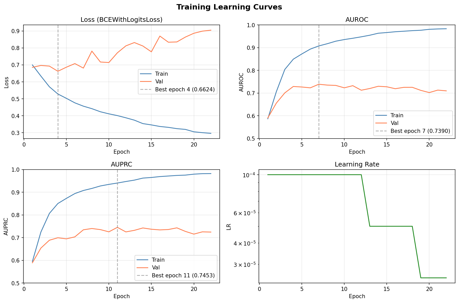
As we can see here, the model achieves a peak validation AUROC of around 0.739 at epoch 7, after which it starts to overfit (training AUROC continues to improve while validation AUROC plateaus and then declines). The learning rate scheduler reduces the learning rate at epoch 13 when the validation AUROC plateaus, but the model still does not improve further, leading to early stopping at epoch 22.
I adjusted the training hyperparameters to mitigate overfitting, such as increasing dropout rates and weight decay, stronger label smoothing, reducing model size, and using a more aggressive learning rate scheduler. However, the model still shows signs of overfitting after a few epochs, which is probably due to the limitation of the data.
Now that we have the best model checkpoint saved, we can load it and evaluate its performance on the held-out test set to see how well it generalizes to unseen data.
model.load_state_dict(torch.load(f"{save_path}/data/best_model.pt"))
model = model.to(device)
model.eval()

_, test_auroc, test_auprc, test_probs, test_labels = evaluate(
    model, test_loader, loss_fn, device
)

from sklearn.metrics import (
    roc_auc_score,
    average_precision_score,
    accuracy_score,
    matthews_corrcoef,
    confusion_matrix,
    PrecisionRecallDisplay,
    RocCurveDisplay,
    f1_score,
    precision_score,
    recall_score
)

# Convert probabilities to binary predictions at 0.5 threshold
test_preds = (test_probs >= 0.5).astype(int)

print(f"AUROC     : {roc_auc_score(test_labels, test_probs):.4f}")
print(f"AUPRC     : {average_precision_score(test_labels, test_probs):.4f}")
print(f"F1 score  : {f1_score(test_labels, test_preds):.4f}")
print(f"Precision : {precision_score(test_labels, test_preds):.4f}")
print(f"Recall    : {recall_score(test_labels, test_preds):.4f}")
print(f"Accuracy  : {accuracy_score(test_labels, test_preds):.4f}")
print(f"MCC       : {matthews_corrcoef(test_labels, test_preds):.4f}")
print(f"Confusion matrix:\n{confusion_matrix(test_labels, test_preds)}")
Output:
AUROC     : 0.7466
AUPRC     : 0.7470
F1 score  : 0.6314
Precision : 0.7195
Recall    : 0.5626
Accuracy  : 0.6717
MCC       : 0.3518
Confusion matrix:
[[705 198]
 [395 508]]
The AUPRC is around 0.75, which is similar, if not slightly higher than the published models. But since the published data used HIPPIE data and this data is HuRI, and that the splitting method may not be exactly the same, it is difficult to determine if this is a real improvement to the models in the paper. However, the Reim et al. models were trained with over 163k training data, while here I only have 47k training data, so achieving similar performance with much less data is probably a good sign that the model architecture and training strategy are effective.
Also, at a decision probability threshold of 0.5, the precision is 0.72, while the recall is only 0.56. This indicates that the model is more accurate in calling true interactions, but the sensitivity of the model in identifying all positive interactions is not great. We can tune the decision threshold as below depending on our downstream requirements (e.g. catering for different wet lab validation strategies).
# Try different thresholds and see how metrics change
from sklearn.metrics import precision_recall_fscore_support, confusion_matrix

thresholds = [0.3, 0.4, 0.5, 0.6]

print(f"{'Threshold':>10} {'Precision':>10} {'Recall':>10} {'F1':>10} {'MCC':>10}")
print("-" * 55)

for thr in thresholds:
    preds = (test_probs >= thr).astype(int)
    p, r, f1, _ = precision_recall_fscore_support(
        test_labels, preds, average='binary', zero_division=0
    )
    mcc = matthews_corrcoef(test_labels, preds)
    print(f"{thr:>10.2f} {p:>10.4f} {r:>10.4f} {f1:>10.4f} {mcc:>10.4f}")
Output:
 Threshold  Precision     Recall         F1        MCC
-------------------------------------------------------
      0.30     0.6599     0.7198     0.6886     0.3503
      0.40     0.6845     0.6224     0.6520     0.3369
      0.50     0.7195     0.5626     0.6314     0.3518
      0.60     0.7479     0.4994     0.5989     0.3511
Plot the PR curve:
display = PrecisionRecallDisplay.from_predictions(
    test_preds, test_labels, name="Precision Recall Curve", plot_chance_level=True, despine=True
)
_ = display.ax_.set_title("2-class Precision-Recall curve")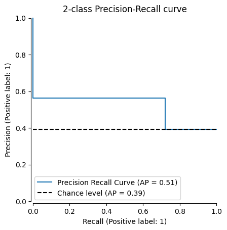
Now, I will compare the performance of the transformer-based model with a simpler Random Forest classifier, using the same embeddings as input features. This will help us understand how much the transformer architecture contributes to the performance compared to a more traditional machine learning model.
Prepare the data for training:
# Convert embeddings to numpy
for key, values in embedding_dict.items():
    embedding_dict[key] = values.numpy()

def prepare_rf_data(df, embedding_dict):
    X = []
    y = []
    for _, row in df.iterrows():
        protein1_emb = embedding_dict[row['Protein1_ID']]
        protein2_emb = embedding_dict[row['Protein2_ID']]
        # Concatenate embeddings to form feature vector
        X.append(np.concatenate((protein1_emb, protein2_emb)))
        y.append(row['Y'])
    return np.array(X), np.array(y)

# Prepare data for all splits
X_train, y_train = prepare_rf_data(train_df, embedding_dict)
X_val, y_val = prepare_rf_data(valid_df, embedding_dict)
X_test, y_test = prepare_rf_data(test_df, embedding_dict)

print(f"Train data shape: {X_train.shape}, {y_train.shape}")
print(f"Validation data shape: {X_val.shape}, {y_val.shape}")
print(f"Test data shape: {X_test.shape}, {y_test.shape}")
Output:
Train data shape: (47306, 2560), (47306,)
Validation data shape: (1832, 2560), (1832,)
Test data shape: (1806, 2560), (1806,)
I use RandomizedSearchCV to find the best hyperparameters for the Random Forest model. I will tune the number of trees (n_estimators) and the number of features to consider at each split (max_features).
from sklearn.ensemble import RandomForestClassifier
from sklearn.model_selection import RandomizedSearchCV
import scipy.stats as stats

# Define the parameter distribution for RandomizedSearchCV
param_dist = {
    'n_estimators': stats.randint(50, 500),         # Number of trees in the forest
    'max_features': ['sqrt', 'log2'],                # Number of features to consider at each split
}

# Initialize a RandomForestClassifier
rf = RandomForestClassifier(random_state=42, n_jobs=-1) # n_jobs=-1 uses all available cores

# Initialize RandomizedSearchCV
# The `scoring` parameter can be set to 'roc_auc' or 'average_precision' for PPI prediction.
# 'average_precision' is often preferred for imbalanced datasets.
random_search = RandomizedSearchCV(
    estimator=rf,
    param_distributions=param_dist,
    n_iter=10,  # Number of parameter settings that are sampled. More is better but takes longer.
    cv=3,       # Number of folds for cross-validation
    scoring='roc_auc', # Evaluate using AUROC
    random_state=42,
    n_jobs=-1,
    verbose=3
)

print("Starting RandomizedSearchCV...")
random_search.fit(X_train, y_train)

print("RandomizedSearchCV completed.")
print(f"Best parameters: {random_search.best_params_}")
print(f"Best AUROC score on training data with cross-validation: {random_search.best_score_:.4f}")
Output:
Starting RandomizedSearchCV...
Fitting 3 folds for each of 10 candidates, totalling 30 fits
[CV 1/3] END max_features=sqrt, n_estimators=320;, score=0.904 total time=10.2min
[CV 3/3] END max_features=sqrt, n_estimators=171;, score=0.900 total time= 5.3min
[CV 2/3] END max_features=sqrt, n_estimators=149;, score=0.904 total time= 4.6min
RandomizedSearchCV completed.
Best parameters: {'max_features': 'sqrt', 'n_estimators': 485}
Best AUROC score on training data with cross-validation: 0.9053
Let’s see how the metrics change with different decision thresholds for the Random Forest model, and then evaluate the best model on the test set.
from sklearn.metrics import (
    roc_auc_score,
    average_precision_score,
    accuracy_score,
    matthews_corrcoef,
    confusion_matrix,
    f1_score,
    precision_score,
    recall_score,
    precision_recall_fscore_support
)

best_rf_model = random_search.best_estimator_

# Predict probabilities on the test set
rf_test_probs = best_rf_model.predict_proba(X_test)[:, 1]

thresholds = [0.3, 0.4, 0.5, 0.6]

print(f"\n{'Threshold':>10} {'Precision':>10} {'Recall':>10} {'F1':>10} {'MCC':>10}")
print("-" * 55)
for thr in thresholds:
    preds = (rf_test_probs >= thr).astype(int)
    p, r, f1, _ = precision_recall_fscore_support(
        y_test, preds, average='binary', zero_division=0
    )
    mcc = matthews_corrcoef(y_test, preds)
    print(f"{thr:>10.2f} {p:>10.4f} {r:>10.4f} {f1:>10.4f} {mcc:>10.4f}")
Output:
 Threshold  Precision     Recall         F1        MCC
-------------------------------------------------------
      0.30     0.5298     0.8472     0.6519     0.1189
      0.40     0.6760     0.3488     0.4602     0.2075
      0.50     0.7273     0.0266     0.0513     0.0620
      0.60     0.5833     0.0078     0.0153     0.0136
I’ll use the 0.4 threshold for the Random Forest model to calculate the final evaluation metrics on the test set, since it gives a better balance between precision and recall compared to the default 0.5 threshold.
# Convert probabilities to binary predictions at 0.4 threshold
rf_test_preds = (rf_test_probs >= 0.4).astype(int)

print("\nRandom Forest Model Evaluation on Test Set:")
print(f"AUROC     : {roc_auc_score(y_test, rf_test_probs):.4f}")
print(f"AUPRC     : {average_precision_score(y_test, rf_test_probs):.4f}")
print(f"F1 score  : {f1_score(y_test, rf_test_preds):.4f}")
print(f"Precision : {precision_score(y_test, rf_test_preds):.4f}")
print(f"Recall    : {recall_score(y_test, rf_test_preds):.4f}")
print(f"Accuracy  : {accuracy_score(y_test, rf_test_preds):.4f}")
print(f"MCC       : {matthews_corrcoef(y_test, rf_test_preds):.4f}")
print(f"Confusion matrix:\n{confusion_matrix(y_test, rf_test_preds)}")
Output:
Random Forest Model Evaluation on Test Set:
AUROC     : 0.6207
AUPRC     : 0.6200
F1 score  : 0.4602
Precision : 0.6760
Recall    : 0.3488
Accuracy  : 0.5908
MCC       : 0.2075
Confusion matrix:
[[752 151]
[588 315]]Although the model built here achieved similar performance to the published models, the accuracy is probably still not ideal for an actual in silico PPI screening campaign. The literature suggested that the performance boost of such model is mostly attributed to the use of pretrained language models like ESM2. Indeed, in this exercise, we can see that the performance gain from the transformer model vs. random forest is significant but not huge, and the model still shows signs of overfitting after a few epochs.
Here are a few potential next steps to further improve performance for PPI prediction:
Finally, it is important to note that the performance of the model is still limited by the quality and quantity of the training data. The current data mostly measure binary interactions, but in reality, the strength of interactions can vary widely. In the living cell, PPI is affected by many factors, including protein stoichiometry, subcellular localization, post-translational modifications, and the presence of other interacting partners. The availability of large-scale Y2H data like HuRI is a great step forward, but it still only captures a fraction of the complex interactome in the cell, and at a specific condition that may or may not be relevant to the biological targets of interest. Therefore, more high-throughput, physiologically relevant PPI data will be needed to further improve the performance of these models and make them more useful for real-world applications.
The codes were written with the aid of Claude Sonnet 4.6 and Gemini 2.5 Flash, and the model training was performed on Google Colab Pro+ with a Tesla T4 GPU. The accuracy of the codes were verified by the author.