From Fingerprints to Message Passing: Benchmarking Three Approaches to Molecular Toxicity Prediction on Tox21

Summary

In this post, I compare three approaches to predicting chemical toxicity directly from molecular structure, using the Tox21 dataset (~7,800 compounds tested across 12 nuclear receptor and stress-response assays). The first is a Random Forest trained on molecular fingerprints, a standard cheminformatics baseline. The second is a Graph Neural Network (GINE) built from scratch that learns directly from atoms and bonds. The third is Chemprop, a widely-used graph neural network package, combined with RDKit 2D molecular descriptors. All three models are evaluated using a scaffold split, which keeps structurally similar molecules out of both the training and test sets for a more realistic test of generalization to new chemical structures. All three models achieve similar performance that aligns with previous literature benchmarks. I also walk through a real numerical pitfall with RDKit descriptors that can silently corrupt training, and use t-SNE to check whether the learned graph representations capture meaningful chemical structure.

Introduction

Tox21 is a multi-task binary classification dataset for predicting the toxicity of chemical compounds. The dataset contains 12 different toxicity tasks, each corresponding to a specific biological target or pathway. The goal is to predict whether a given compound is toxic or non-toxic for each of these tasks. Each compound is represented by its SMILES string (Chemprop additionally uses RDKit 2D descriptors as extra molecule-level features, described in Model 3). The dataset is highly imbalanced, with some tasks having very few positive examples (3-15% positive rates). There are also many missing labels. This provides a challenge for training machine learning models. We will tackle these problems by using specific metrics and loss function as described later.

Three models to train:

1. Random Forest (RF) with ECFP2048 (Morgan fingerprints) as input features: this is considered as a baseline model with classical machine learning approach trained on molecular fingerprints. The RF model will be well-tuned with hyperparameter search and cross-validation.

2. GINE (Graph Isomorphism Network with Edge features), trained directly on atom- and bond-level graph features: GIN or GINE is a type of Graph Neural Network (GNN) with message-passing similar to a Graph Convolution Network (GCN). Unlike GCN, which combines messages by averaging neighbors’ embeddings, GINE sums the neighboring messages instead, which better preserves information about the number of neighbors a node has. This allows for better differentiation of certain non-isomorphic graphs than GCN. For an introduction into GIN vs GCN, see the TeachOpenCADD GNN tutorial. The GINE model will be built from scratch using PyG’s GINEConv - a variant of GIN that includes both node and edge features during the message-passing steps (a typical GIN only calculates node features). This allows for learning of molecular properties from both atom and bond features from the compounds. I will be using the PyTorch Geometric (PyG) library to build the GINE model from scratch.

3. Chemprop (D-MPNN), trained on the molecular graph plus RDKit 2D (whole-molecule) descriptors as extra features: Chemprop is a high-level library for building and training D-MPNN (Directed Message Passing Neural Network) models to predict molecular properties. D-MPNN passes messages along directed bonds and explicitly excludes the reverse-direction message when aggregating each edge’s update, avoiding the “tottering” problem (a signal bouncing immediately back to the atom it came from). D-MPNN has been shown to perform well on larger industrial proprietary datasets. Chemprop combines D-MPNN with a feed-forward neural network (FFNN) that takes in additional molecular features, such as RDKit 2D features, to improve the model’s performance. Chemprop abstracts away the details of building and training D-MPNN models, making it easier to use. I will be using Chemprop’s Python-first API that is built on PyTorch Lightning to train the D-MPNN model.

To prevent data leakage, a scaffold split will be performed on the Tox21 dataset, which ensures that structurally related molecules do not end up in different partitions (train/validation/test). This is important because if structurally similar molecules are present in both training and test sets, the model may perform well on the test set simply because it has seen similar molecules during training, rather than learning to generalize to unseen molecules.

The final performance of each model will be summarized using AUROC, AUPRC and binary cross-entropy (BCE) loss. It is important to note that the RF model will be well-tuned with hyperparameter search and cross-validation, while the GINE and Chemprop models will be trained once with pre-selected hyperparameters. The learned graph-level embeddings from the GINE and Chemprop models will be visualized using t-SNE to see if the embeddings capture any meaningful chemical and predictive properties in the data.

Data processing

Loading required libraries and setting up the environment:

import numpy as np
import pandas as pd
import matplotlib.pyplot as plt
import seaborn as sns

import torch
import torch.nn as nn
import torch.nn.functional as F
from torch_geometric.data import Data, Dataset
from torch_geometric.loader import DataLoader as PyGDataLoader
from torch_geometric.nn import GINEConv, global_mean_pool, global_max_pool

from rdkit import Chem
from rdkit.Chem import Descriptors, Crippen, rdMolDescriptors, rdFingerprintGenerator

from sklearn.ensemble import RandomForestClassifier
from sklearn.model_selection import RandomizedSearchCV, StratifiedKFold
from sklearn.metrics import roc_auc_score, average_precision_score, log_loss
from sklearn.manifold import TSNE

from rdkit.Chem.Scaffolds import MurckoScaffold

from lightning import pytorch as pl
from lightning.pytorch.callbacks import EarlyStopping, ModelCheckpoint, LearningRateMonitor
from lightning.pytorch.loggers import CSVLogger

from chemprop import data as cp_data
from chemprop import featurizers as cp_featurizers
from chemprop import models as cp_models
from chemprop import nn as cp_nn
from chemprop import utils as cp_utils

DEVICE = torch.device("cuda" if torch.cuda.is_available() else "cpu")
SEED = 524
np.random.seed(SEED)
torch.manual_seed(SEED)

Scaffold split

The following functions generate Bemis-Murcko scaffolds and perform the scaffold split on the Tox21 dataset:

def generate_scaffold(smiles, include_chirality=False):
    mol = Chem.MolFromSmiles(smiles)
    return MurckoScaffold.MurckoScaffoldSmiles(mol=mol, includeChirality=include_chirality)

def scaffold_split(smiles_list, frac_train=0.8, frac_valid=0.1, frac_test=0.1, seed=SEED):
    """
    Bemis-Murcko scaffold split: group molecules by scaffold, assign whole groups to
    train/valid/test (largest groups first into train), so structurally related molecules
    never end up split across partitions. Equivalent to DeepChem's ScaffoldSplitter.
    """
    assert abs(frac_train + frac_valid + frac_test - 1.0) < 1e-6
    rng = np.random.RandomState(seed)

    scaffold_to_indices = {}
    for idx, smi in enumerate(smiles_list):
        scaffold = generate_scaffold(smi)
        scaffold_to_indices.setdefault(scaffold, []).append(idx) # e.g. {"c1ccccc1": [0, 2], "c1ccncc1": [1]}

    # Shuffle within same-size groups for reproducible tie-breaking, then sort by group
    # size descending (largest scaffold groups placed first).
    groups = list(scaffold_to_indices.values())
    rng.shuffle(groups)
    groups.sort(key=len, reverse=True)

    n_total = len(smiles_list)
    n_train_cutoff = frac_train * n_total
    n_valid_cutoff = (frac_train + frac_valid) * n_total

    train_idx, valid_idx, test_idx = [], [], []
    for group in groups:
        if len(train_idx) + len(group) <= n_train_cutoff:
            train_idx.extend(group)
        elif len(train_idx) + len(valid_idx) + len(group) <= n_valid_cutoff:
            valid_idx.extend(group)
        else:
            test_idx.extend(group)

    return np.array(train_idx), np.array(valid_idx), np.array(test_idx)

TOX21_TASKS = [
    'NR-AR', 'NR-AR-LBD', 'NR-AhR', 'NR-Aromatase', 'NR-ER', 'NR-ER-LBD',
    'NR-PPAR-gamma', 'SR-ARE', 'SR-ATAD5', 'SR-HSE', 'SR-MMP', 'SR-p53'
]
N_TASKS = len(TOX21_TASKS)
TOX21_URL = "https://deepchemdata.s3-us-west-1.amazonaws.com/datasets/tox21.csv.gz"

raw_df = pd.read_csv(TOX21_URL, compression="gzip")
print("raw rows:", len(raw_df))

# Drop the small number of molecules RDKit can't parse (invalid valence etc.)
parses_ok = raw_df["smiles"].apply(lambda s: Chem.MolFromSmiles(s) is not None)
print(f"\ndropping {(~parses_ok).sum()} unparseable SMILES out of {len(raw_df)}")
raw_df = raw_df[parses_ok].reset_index(drop=True)

all_smiles = raw_df["smiles"].values
y_all = raw_df[TOX21_TASKS].values.astype(np.float32)   # NaN where missing
w_all = (~np.isnan(y_all)).astype(np.float32)            # 1 = present, 0 = missing
y_all = np.nan_to_num(y_all, nan=0.0)                     # garbage fill where w==0

train_idx, val_idx, test_idx = scaffold_split(all_smiles, frac_train=0.8, frac_valid=0.1, frac_test=0.1, seed=SEED)

def subset(idx):
    return all_smiles[idx], y_all[idx], w_all[idx]

train_smiles, y_train, w_train = subset(train_idx)
val_smiles,   y_val,   w_val   = subset(val_idx)
test_smiles,  y_test,  w_test  = subset(test_idx)

print(f"\ntrain / val / test molecules: {len(train_smiles)} / {len(val_smiles)} / {len(test_smiles)}")

Output:

dropping 8 unparseable SMILES out of 7831

train / val / test molecules: 6258 / 782 / 783

EDA

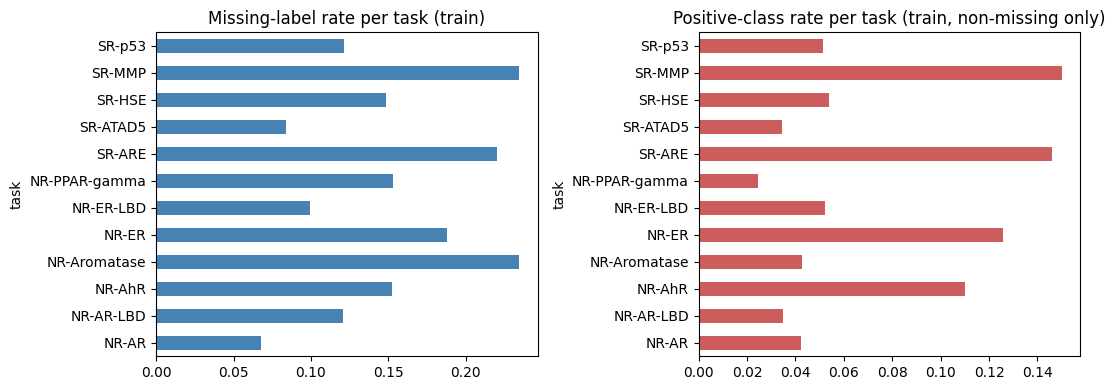
To get a quick overview of the dataset, we can visualize the missing-label rate and positive-class rate for each task in the training set:

# Quick EDA: missing-label rate and positive-class rate per task (on non-missing labels)
rows = []
for i, t in enumerate(TOX21_TASKS):
    mask = w_train[:, i] > 0
    missing_rate = 1 - mask.mean()
    pos_rate = y_train[mask, i].mean() if mask.sum() > 0 else np.nan
    rows.append({"task": t, "missing_rate_train": missing_rate, "positive_rate_train": pos_rate})
eda_df = pd.DataFrame(rows).set_index("task")

fig, ax = plt.subplots(1, 2, figsize=(11, 4))
eda_df["missing_rate_train"].plot.barh(ax=ax[0], color="steelblue")
ax[0].set_title("Missing-label rate per task (train)")
eda_df["positive_rate_train"].plot.barh(ax=ax[1], color="indianred")
ax[1].set_title("Positive-class rate per task (train, non-missing only)")
plt.tight_layout()
plt.show()

As we can see, the Tox21 dataset is highly imbalanced, with some tasks having very few positive examples. There are also many missing labels. We will deal with these problems by including metrics that are robust to class imbalance (AUPRC) and by using a loss function that ignores missing labels. To that end, both AUROC and AUPRC will be computed per task and then macro-averaged across tasks. The loss function will be a masked binary cross-entropy loss, which ignores missing labels during training.

Model 1: Random Forest

Extracting ECFP2048 features

ECFP2048, which is also known as Morgan fingerprints with radius 2, is a widely used molecular fingerprint representation in cheminformatics. It captures the presence of substructures in molecules and is particularly useful for machine learning tasks involving chemical data. Here we will use the bit vector representation of ECFP2048 as input features for a Random Forest classifier. Since Tox21 is a multi-task dataset with missing labels for some tasks, we will train 12 independent Random Forest classifiers, one for each task. Each classifier will be trained only on the rows where that task’s label is present.

def ecfp_features(smiles_list, radius=2, n_bits=2048):
    morgan_gen = rdFingerprintGenerator.GetMorganGenerator(radius=radius, fpSize=n_bits)
    fps = np.zeros((len(smiles_list), n_bits), dtype=np.float32) # (N, 2048)
    valid = np.ones(len(smiles_list), dtype=bool) # (N,) of True
    for i, smi in enumerate(smiles_list):
        mol = Chem.MolFromSmiles(smi)
        if mol is None:
            valid[i] = False
            continue
        fps[i] = morgan_gen.GetFingerprintAsNumPy(mol).astype(np.float32)
    return fps, valid

X_train_ecfp, valid_train = ecfp_features(train_smiles)
X_val_ecfp,   valid_val   = ecfp_features(val_smiles)
X_test_ecfp,  valid_test  = ecfp_features(test_smiles)
print("ECFP2048 feature matrices:", X_train_ecfp.shape, X_val_ecfp.shape, X_test_ecfp.shape)
print("Unparseable SMILES (train/val/test):", (~valid_train).sum(), (~valid_val).sum(), (~valid_test).sum())

Output:

ECFP2048 feature matrices: (6258, 2048) (782, 2048) (783, 2048)
Unparseable SMILES (train/val/test): 0 0 0

Model training and evaluation

from scipy import stats

RF_PARAM_DIST = {
    "n_estimators": stats.randint(50, 400),
    "max_depth": [10, 20, 30, None], # keep a depth cap in the mix — controls fit time, tree size, and overfitting
    "max_features": ["sqrt", "log2"],
    "class_weight": ["balanced", None], # RF's class weight balancing for imbalanced target
}

def fit_rf_for_task(X_tr, y_tr, mask_tr, n_iter=20, cv=3, seed=SEED, refit_metric="average_precision"):
    m = mask_tr > 0
    X, y = X_tr[m], y_tr[m].astype(int)
    cv_splitter = StratifiedKFold(n_splits=cv, shuffle=True, random_state=seed)
    scoring = {"roc_auc": "roc_auc", "average_precision": "average_precision"} # both AUROC and AUPRC due to imbalanced data
    search = RandomizedSearchCV(
        RandomForestClassifier(random_state=seed, n_jobs=1),   # single-threaded trees — avoids oversubscription (if -1 will be very slow)
        param_distributions=RF_PARAM_DIST,
        n_iter=n_iter, cv=cv_splitter, scoring=scoring,
        refit=refit_metric, random_state=seed, n_jobs=-1,      # parallelism lives here instead
    )
    search.fit(X, y)
    best_idx = search.best_index_
    cv_auroc = search.cv_results_["mean_test_roc_auc"][best_idx]
    cv_auprc = search.cv_results_["mean_test_average_precision"][best_idx]
    return search.best_estimator_, search.best_params_, cv_auroc, cv_auprc

rf_models, rf_best_params = {}, {}
for i, task in enumerate(TOX21_TASKS):
    model, params, cv_auroc, cv_auprc = fit_rf_for_task(X_train_ecfp, y_train[:, i], w_train[:, i])
    rf_models[task] = model
    rf_best_params[task] = params
    print(f"[{task}] CV auroc={cv_auroc:.3f} auprc={cv_auprc:.3f} | best params: {params}")

rf_best_params_df = pd.DataFrame(rf_best_params).T
rf_best_params_df.index.name = "tasks"
print(rf_best_params_df)

Output:

              class_weight max_depth max_features n_estimators
tasks                                                         
NR-AR                 None        20         log2          396
NR-AR-LBD         balanced        20         sqrt          333
NR-AhR                None        30         log2          231
NR-Aromatase          None        20         log2          396
NR-ER             balanced        20         sqrt          333
NR-ER-LBD         balanced        30         sqrt          228
NR-PPAR-gamma         None        30         log2          231
SR-ARE            balanced      None         sqrt          393
SR-ATAD5              None        20         log2          399
SR-HSE                None        30         sqrt          260
SR-MMP            balanced      None         sqrt          393
SR-p53                None        30         log2          231

Now evaluate the Random Forest models on the validation and test sets, computing AUROC, AUPRC, and binary cross-entropy (BCE) per task, and then macro-averaging across tasks:

def masked_task_metrics(y_true_2d, y_prob_2d, w_2d, task_names):
    """
    Output metrics for multi-label binary classification.
    y_prob_2d: prediction probability (not logits)
    w_2d: 1=present, 0=missing
    task_names: list of task names
    Returns: 
      df: metrics per task
      macro: macro-averaged metrics
    """
    rows = []
    for i, t in enumerate(task_names):
        m = w_2d[:, i] > 0
        yt, yp = y_true_2d[m, i], y_prob_2d[m, i]
        if m.sum() == 0 or len(np.unique(yt)) < 2:
            rows.append({"task": t, "n_not_missing": int(m.sum()), "auroc": np.nan, "auprc": np.nan, "bce": np.nan})
            continue
        eps = 1e-7
        yp_clip = np.clip(yp, eps, 1 - eps) # clip to prevent log(0)
        rows.append({
            "task": t, "n_not_missing": int(m.sum()),
            "auroc": roc_auc_score(yt, yp),
            "auprc": average_precision_score(yt, yp),
            "bce": log_loss(yt, yp_clip, labels=[0, 1]),
        })
    df = pd.DataFrame(rows).set_index("task")
    macro = df[["auroc", "auprc", "bce"]].mean(skipna=True)
    return df, macro

def rf_predict_proba_matrix(models, X, task_names):
    P = np.zeros((X.shape[0], len(task_names)), dtype=np.float32)
    for i, t in enumerate(task_names):
        P[:, i] = models[t].predict_proba(X)[:, 1]
    return P

rf_val_proba  = rf_predict_proba_matrix(rf_models, X_val_ecfp,  TOX21_TASKS)
rf_test_proba = rf_predict_proba_matrix(rf_models, X_test_ecfp, TOX21_TASKS)

rf_val_per_task,  rf_val_macro  = masked_task_metrics(y_val,  rf_val_proba,  w_val,  TOX21_TASKS)
rf_test_per_task, rf_test_macro = masked_task_metrics(y_test, rf_test_proba, w_test, TOX21_TASKS)

print("RF — validation macro:\n", rf_val_macro, "\n")
print("RF — test macro:\n", rf_test_macro)

Output:

RF — validation macro:
 auroc    0.741988
auprc    0.392214
bce      0.290596
dtype: float64 

RF — test macro:
 auroc    0.732228
auprc    0.382328
bce      0.287920
dtype: float64

print(rf_test_per_task)

Output:

               n_not_missing     auroc     auprc       bce
task                                                      
NR-AR                    710  0.662598  0.444872  0.140264
NR-AR-LBD                625  0.825365  0.470748  0.175261
NR-AhR                   631  0.810336  0.480379  0.339632
NR-Aromatase             513  0.750583  0.413734  0.287437
NR-ER                    542  0.700920  0.434790  0.470501
NR-ER-LBD                654  0.749201  0.391579  0.186523
NR-PPAR-gamma            573  0.715393  0.230247  0.148016
SR-ARE                   461  0.728359  0.455434  0.532457
SR-ATAD5                 666  0.738581  0.198776  0.198404
SR-HSE                   564  0.562813  0.150229  0.281093
SR-MMP                   517  0.806099  0.589835  0.384019
SR-p53                   633  0.736491  0.327309  0.311428

Model 2: GINE

Extracting atom and bond features

Extracting atom and bond features from the SMILES strings using RDKit, and converting them into PyTorch Geometric Data objects:

ATOM_LIST = ['C', 'N', 'O', 'S', 'F', 'Si', 'P', 'Cl', 'Br', 'Mg', 'Na', 'Ca', 'Fe',
             'As', 'I', 'B', 'V', 'K', 'Tl', 'Sn', 'Sb', 'Se', 'Zn', 'Other']
HYBRIDIZATIONS = [Chem.rdchem.HybridizationType.SP, Chem.rdchem.HybridizationType.SP2,
                   Chem.rdchem.HybridizationType.SP3, Chem.rdchem.HybridizationType.SP3D,
                   Chem.rdchem.HybridizationType.SP3D2, 'Other']
CHIRAL_TAGS = [Chem.rdchem.ChiralType.CHI_UNSPECIFIED, Chem.rdchem.ChiralType.CHI_TETRAHEDRAL_CW,
               Chem.rdchem.ChiralType.CHI_TETRAHEDRAL_CCW, 'Other']
BOND_TYPES = [Chem.rdchem.BondType.SINGLE, Chem.rdchem.BondType.DOUBLE,
              Chem.rdchem.BondType.TRIPLE, Chem.rdchem.BondType.AROMATIC]
STEREO_TYPES = [Chem.rdchem.BondStereo.STEREONONE, Chem.rdchem.BondStereo.STEREOZ,
                 Chem.rdchem.BondStereo.STEREOE, 'Other']

def one_hot(x, choices: list) -> list[int]:
    v = [0] * len(choices)
    idx = choices.index(x) if x in choices else len(choices) - 1
    v[idx] = 1
    return v

def atom_features(atom: Chem.rdchem.Atom) -> np.ndarray:
    """
    Returns a bit vector of atom features.
    atom: RDKit atom object (from Mol object)
    returns: 1D np.array of atom features with shape (52,)
    """
    return np.array(
        one_hot(atom.GetSymbol(), ATOM_LIST) +
        one_hot(atom.GetTotalDegree(), [0, 1, 2, 3, 4, 5]) +
        one_hot(atom.GetFormalCharge(), [-2, -1, 0, 1, 2]) +
        one_hot(atom.GetHybridization(), HYBRIDIZATIONS) +
        one_hot(atom.GetTotalNumHs(), [0, 1, 2, 3, 4]) +
        one_hot(atom.GetChiralTag(), CHIRAL_TAGS) +
        [int(atom.GetIsAromatic()), int(atom.IsInRing())],
        dtype=np.float32,
    )

def bond_features(bond: Chem.rdchem.Bond) -> np.ndarray:
    """
    Returns a bit vector of bond features.
    bond: RDKit bond object (from BondList object)
    returns: 1D np.array of bond features with shape (10,)
    """
    return np.array(
        one_hot(bond.GetBondType(), BOND_TYPES) +
        one_hot(bond.GetStereo(), STEREO_TYPES) +
        [int(bond.GetIsConjugated()), int(bond.IsInRing())],
        dtype=np.float32,
    )

def mol_to_pyg_data(smiles: str,
                    y: np.ndarray | None = None,
                    w: np.ndarray | None = None
                    ) -> Data | None:
    """
    Converts a SMILES string into a PyTorch Geometric Data object.

    Args:
      smiles: The SMILES string of the molecule.
      y: Optional target labels (e.g., toxicity values) for the molecule.
      w: Optional weights/mask for the target labels (1 for present, 0 for missing).

    Returns:
      A PyTorch Geometric Data object representing the molecule, or None if the SMILES
      string cannot be parsed or results in a molecule with no atoms.
    """
    mol = Chem.MolFromSmiles(smiles)
    if mol is None or mol.GetNumAtoms() == 0:
        return None
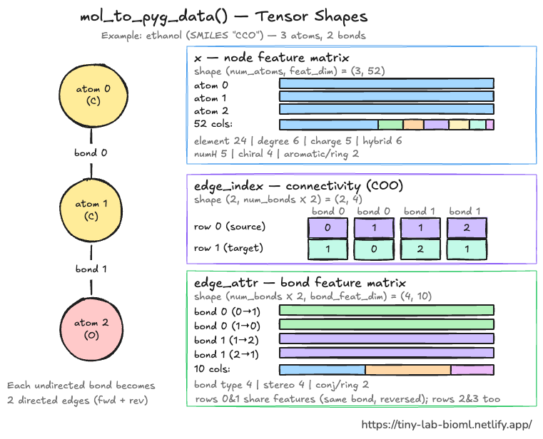
    x = torch.tensor(np.stack([atom_features(a) for a in mol.GetAtoms()]), dtype=torch.float)
    # x is node features of shape: (num_nodes_in_molecule, num_node_features)

    edge_index, edge_attr = [], []
    for bond in mol.GetBonds():
        i, j = bond.GetBeginAtomIdx(), bond.GetEndAtomIdx()
        bf = bond_features(bond)
        edge_index += [[i, j], [j, i]]
        edge_attr += [bf, bf]
    if len(edge_index) == 0:  # single-atom molecule edge case, no bonds (e.g. bare ions like [Na+])
        edge_index = torch.empty((2, 0), dtype=torch.long)
        # PyG expects shape (2, num_edges), so empty (2, 0) is start/end nodes with no edges
        # torch.long gives int64
        edge_attr = torch.empty((0, BOND_FEAT_DIM), dtype=torch.float)
        # Gives empty edge_attr shape (0, 10)
    else:
        edge_index = torch.tensor(edge_index, dtype=torch.long).t().contiguous()
        # If a atom has N bonds -> edge index will be: (2, 2 * N), which is:
        # (StartAtom/EndAtom, i:j/j:i * N bonds)
        edge_attr = torch.tensor(np.stack(edge_attr), dtype=torch.float)
        # edge_attr output: (2 * N bonds, 10)

        """
        Demo: 
        edge_index = [[1, 2], [2, 1], [3, 4], [4, 3]]
        In [29]: torch.tensor(edge_index, dtype=torch.long)
        Out[29]:
        tensor([[1, 2],
                [2, 1],
                [3, 4],
                [4, 3]])
        In [30]: torch.tensor(edge_index, dtype=torch.long).t()
        Out[30]:
        tensor([[1, 2, 3, 4],
                [2, 1, 4, 3]])
        """

    # PyG Data object aggregates all the information for a single graph into one container
    data = Data(x=x, edge_index=edge_index, edge_attr=edge_attr, smiles=smiles)
    if y is not None:
        data.y = torch.tensor(y, dtype=torch.float).view(1, -1)
        data.mask = torch.tensor(w, dtype=torch.float).view(1, -1)
    return data

ATOM_FEAT_DIM = len(atom_features(Chem.MolFromSmiles("CCO").GetAtomWithIdx(0)))
BOND_FEAT_DIM = len(bond_features(Chem.MolFromSmiles("CCO").GetBondWithIdx(0)))
print("atom feature dim:", ATOM_FEAT_DIM, "| bond feature dim:", BOND_FEAT_DIM)

Output:

atom feature dim: 52 | bond feature dim: 10

Building PyG data

The PyG Data structure can be summarized as below, using ethanol as an example:

def build_pyg_list(smiles_arr: np.ndarray,
                   y_arr: np.ndarray,
                   w_arr: np.ndarray
                   ) -> list[Data]:
    out = []
    for smi, y, w in zip(smiles_arr, y_arr, w_arr):
        d = mol_to_pyg_data(smi, y, w)
        if d is not None:
            out.append(d)
    return out

# This generates a list of PyG Data objects
# For larger datasets needing on-disk caching, the Dataset subclass is required
train_graphs = build_pyg_list(train_smiles, y_train, w_train)
val_graphs = build_pyg_list(val_smiles, y_val, w_val)
test_graphs = build_pyg_list(test_smiles, y_test, w_test)
print(f"PyG graphs — train/val/test: {len(train_graphs)}/{len(val_graphs)}/{len(test_graphs)}")

BATCH_SIZE = 64
train_loader = PyGDataLoader(train_graphs, batch_size=BATCH_SIZE, shuffle=True)
val_loader = PyGDataLoader(val_graphs, batch_size=BATCH_SIZE, shuffle=False)
test_loader = PyGDataLoader(test_graphs, batch_size=BATCH_SIZE, shuffle=False)

Output:

PyG graphs — train/val/test: 6258/782/783

Message passing in GINE

How is message-passing performed in GINE?

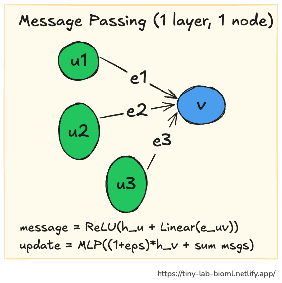
The edge features (here 10 dim) get projected up to match the node features’ working dimension — the 128-dim hidden representation after atom_proj. Once projected to the same dimension, the node and edge features can be combined and passed through a ReLU activation function. This is done for each neighbor u of a given node v, then the messages from all neighbors are summed to get an aggregated message. Finally, this aggregated neighbor message is summed with the feature of node v at a defined proportion, and then passed through an MLP to get the updated node v feature. This can be depicted as follows:

For each neighbor u of node v:
  message(u→v) = ReLU( h_u + Linear(e_uv) )    
Aggregate message:
  aggr(v) = sum over all neighbors u of message(u→v)
Update embed + MLP transformation: 
  h_v_new = MLP( (1 + eps) * h_v + aggr(v) )

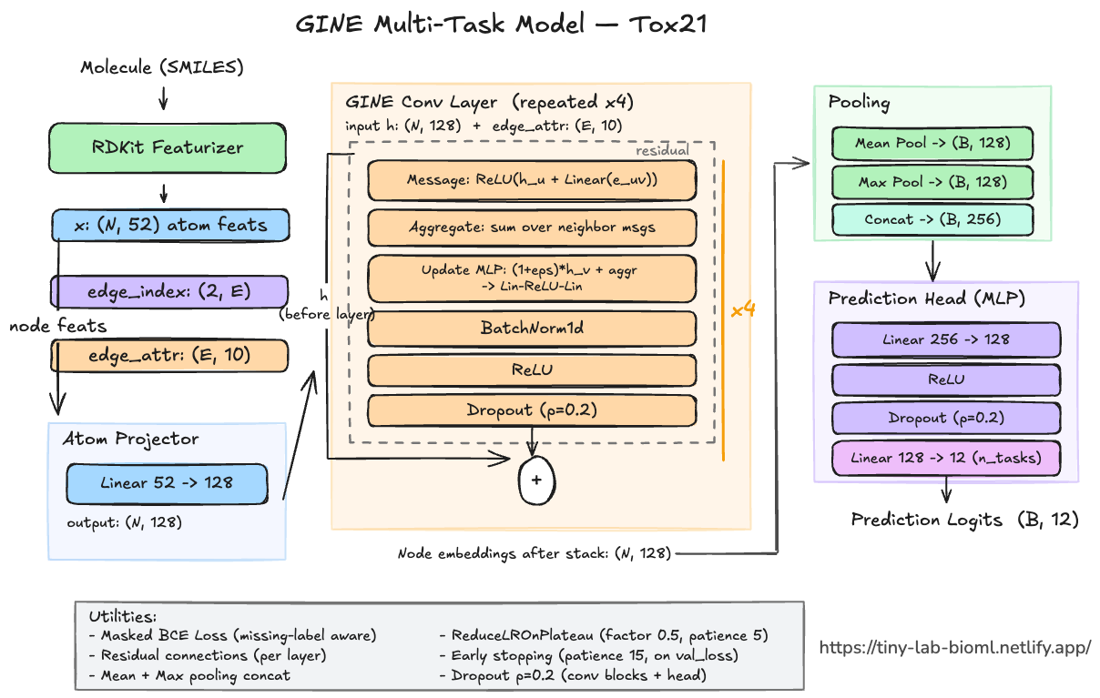
This message-passing is done many times (here 4 layers) to transfer messages across the molecule. One danger of too many layers is “over-smoothing”, when the useful signals get washed out from extensive summing and pooling. A residual connection (h = h + h_new) is added to prevent this and to allow useful signals passing directly through the layers.

The model can be visualized as below:

At the pooling layer, the mean pooled and max pooled features are concatenated to form a graph-level embedding. The max pooled features allow for capturing the most prominent features in the molecule, while the mean pooled features capture the overall distribution of features. The concatenated graph-level embedding is then passed through a MLP to produce the final predictions for each task.

Constructing model

Now we build the model:

class GINEMultiTask(nn.Module):
    def __init__(self,
                 atom_feat_dim,
                 bond_feat_dim,
                 hidden_dim = 128,
                 num_layers = 4,
                 n_tasks = N_TASKS,
                 dropout = 0.2):
        super().__init__()
        self.atom_proj = nn.Linear(atom_feat_dim, hidden_dim)
        self.convs = nn.ModuleList()
        self.bns = nn.ModuleList()
        for _ in range(num_layers):
            mlp = nn.Sequential(
                nn.Linear(hidden_dim, hidden_dim * 2),
                nn.ReLU(),
                nn.Linear(hidden_dim * 2, hidden_dim),
            )
            self.convs.append(GINEConv(mlp, edge_dim=bond_feat_dim))
            self.bns.append(nn.BatchNorm1d(hidden_dim))
        self.dropout = dropout
        pooled_dim = hidden_dim * 2  # mean + max concat
        self.head = nn.Sequential(
            nn.Linear(pooled_dim, hidden_dim),
            nn.ReLU(),
            nn.Dropout(dropout),
            nn.Linear(hidden_dim, n_tasks),
        )

    def embed(self, x, edge_index, edge_attr, batch):
        """
        embed as a separate module to call model.embed() to easily get graph-level
        embeddings for downstream tasks like t-SNE below.
        This is the actual message passing step.
        """
        h = self.atom_proj(x)
        for conv, bn in zip(self.convs, self.bns):
            h_new = conv(h, edge_index, edge_attr)
            h_new = bn(h_new)
            h_new = F.relu(h_new) # nn.F: for cleaner stateless ops within loop
            h_new = F.dropout(h_new, p=self.dropout, training=self.training) # dropout will turn off when eval
            h = h + h_new  # residual connection
        h_mean = global_mean_pool(h, batch) # (B, hidden_dim)
        h_max = global_max_pool(h, batch) # batch: idx of which molecule each atom belongs to
        return torch.cat([h_mean, h_max], dim=1) # (B, hidden_dim * 2)

    def forward(self, x, edge_index, edge_attr, batch):
        embedding = self.embed(x, edge_index, edge_attr, batch)
        return self.head(embedding)

def masked_bce_loss(logits, y, mask):
    """
    Computes the mean binary cross entropy loss for non-missing samples.
    """
    loss_mat = F.binary_cross_entropy_with_logits(logits, y, reduction="none")
    # reduction="none" keeps the full (B, n_tasks) matrix of per-example-per-task losses instead of collapsing it
    loss_mat = loss_mat * mask
    return loss_mat.sum() / mask.sum().clamp(min=1.0) # (summed loss / total sample n) = mean loss

"""
One subtlety worth flagging: this normalizes globally across the whole batch×task matrix,
not per-task. So a task with a low missing-rate (e.g. NR-AhR) contributes more total
loss mass per batch than a sparse one (e.g. NR-AR-LBD), simply because it has more
valid entries — the loss doesn't explicitly rebalance for that. If we ever see the model
doing noticeably worse on the sparsest tasks specifically, that's one place to look
(a per-task-then-averaged loss would be the fix).
"""

💡A note for how PyG handles variable sized molecules with different atom and bond sizes:

The DataLoader actually concatenates everything in a batch into one big disjoint graph. It is the edge index that tells the model that atoms from different molecules do not connect and should not message-pass. At the end of message-passing, per-graph/molecule level feature is calculated by pooling all node features from the same molecule. So how does the model know which nodes belong to which molecule? It gets that information from the batch vector provided.

As an example: say a batch contains an ethanol example (3 atoms, 2 bonds → 4 directed edges) plus a second molecule, methanol (2 atoms, 1 bond → 2 directed edges). PyGDataLoader doesn’t pad anything — it concatenates everything into one big graph:

- x: ethanol's 3 rows stacked on top of methanol's 2 rows  → (5, atom_feat_dim)
- edge_attr: ethanol's 4 rows stacked on top of methanol's 2 rows  → (6, bond_feat_dim))
- edge_index: ethanol's indices unchanged: [[0,1,1,2],[1,0,2,1]]
- methanol's indices shifted by +3 (ethanol's atom count): original methanol edges [[0,1],[1,0]] become [[3,4],[4,3]]
- concatenated: [[0,1,1,2,3,4],[1,0,2,1,4,3]] → shape (2, 6)
- batch: [0,0,0,1,1]   ← which molecule each of the 5 nodes belongs to.

Model training

Next is to design the training loop. We will employ these mechanisms to counter over-fitting:

• Dropout (0.2) inside every conv block and the FFN head.
• ReduceLROnPlateau scheduler on validation loss (halves LR after 5 stagnant epochs).
• Early stopping on validation loss (patience 15), restoring the best-val-loss weights at the end rather than using the final epoch’s weights.
• Weight decay (L2 regularization) in the optimizer.

@torch.no_grad()
def evaluate_gine(model, loader, task_names):
    model.eval()
    all_logits, all_y, all_mask = [], [], []
    total_loss, total_count = 0.0, 0
    for batch in loader:
        batch = batch.to(DEVICE)
        logits = model(batch.x, batch.edge_index, batch.edge_attr, batch.batch)
        y = batch.y.view(-1, len(task_names)) # (B, N_TASKS)
        mask = batch.mask.view(-1, len(task_names))
        loss = masked_bce_loss(logits, y, mask) # this gets avg loss per batch
        total_loss += loss.item() * mask.sum().item() # avg loss X total n
        total_count += mask.sum().item()
        all_logits.append(logits.cpu())
        all_y.append(y.cpu())
        all_mask.append(mask.cpu())
    logits = torch.cat(all_logits).numpy() # concat list of batches[(B,), (B,), ...] -> [N, ]
    y = torch.cat(all_y).numpy()
    mask = torch.cat(all_mask).numpy()
    proba = 1 / (1 + np.exp(-logits)) # sigmoid function
    per_task_metrics, macro_metrics = masked_task_metrics(y, proba, mask, task_names)
    avg_loss = total_loss / max(total_count, 1)
    return avg_loss, macro_metrics, per_task_metrics, proba

def train_gine(model,
               train_loader,
               val_loader,
               task_names,
               max_epochs=100,
               lr=1e-4,
               weight_decay=1e-3,
               patience=15):

    model = model.to(DEVICE)

    optimizer = torch.optim.AdamW(model.parameters(), lr=lr, weight_decay=weight_decay)
    scheduler = torch.optim.lr_scheduler.ReduceLROnPlateau(
        optimizer,
        mode="min", # goal is min val loss
        factor=0.5,
        patience=5,
        min_lr=1e-6
    )

    history = {"train_loss": [],
               "val_loss": [],
               "train_auroc": [],
               "val_auroc": [],
               "lr": []
               }

    best_val_loss, best_state, epochs_no_improve = float("inf"), None, 0

    for epoch in range(1, max_epochs + 1):
        model.train()
        for batch in train_loader:
            batch = batch.to(DEVICE)
            optimizer.zero_grad()
            logits = model(batch.x, batch.edge_index, batch.edge_attr, batch.batch)
            y = batch.y.view(-1, len(task_names))
            mask = batch.mask.view(-1, len(task_names))
            loss = masked_bce_loss(logits, y, mask)
            loss.backward()
            optimizer.step()

        # Generate metrics
        train_loss, train_macro, _, _ = evaluate_gine(model, train_loader, task_names)
        val_loss, val_macro, _, _ = evaluate_gine(model, val_loader, task_names)

        current_lr = optimizer.param_groups[0]["lr"]

        # Log metrics
        history["train_loss"].append(train_loss)
        history["val_loss"].append(val_loss)
        history["train_auroc"].append(train_macro["auroc"])
        history["val_auroc"].append(val_macro["auroc"])
        history["lr"].append(current_lr)

        # Lr scheduling and early stopping
        scheduler.step(val_loss)

        if val_loss < best_val_loss - 1e-4:
            best_val_loss = val_loss
            best_state = {k: v.detach().cpu().clone() for k, v in model.state_dict().items()}
            epochs_no_improve = 0
        else:
            epochs_no_improve += 1

        if epoch % 5 == 0 or epoch == 1:
            print(f"epoch {epoch:3d} | train_loss {train_loss:.4f} | val_loss {val_loss:.4f} "
                  f"| train_auroc {train_macro['auroc']:.4f} | val_auroc {val_macro['auroc']:.4f} "
                  f"| lr {current_lr:.2e}")

        if epochs_no_improve >= patience:
            print(f"Early stopping at epoch {epoch} (no val_loss improvement for {patience} epochs).")
            break

    if best_state is not None:
        model.load_state_dict(best_state)
    return model, history
  
# Instantiate the model
gine_model = GINEMultiTask(ATOM_FEAT_DIM,
                           BOND_FEAT_DIM,
                           hidden_dim=128,
                           num_layers=4,
                           dropout=0.2)

# Training
gine_model, gine_history = train_gine(gine_model,
                                      train_loader,
                                      val_loader,
                                      TOX21_TASKS)

Output:

epoch   1 | train_loss 0.2247 | val_loss 0.2883 | train_auroc 0.6957 | val_auroc 0.6603 | lr 1.00e-04
epoch   5 | train_loss 0.1922 | val_loss 0.2679 | train_auroc 0.8202 | val_auroc 0.7333 | lr 1.00e-04
epoch  10 | train_loss 0.1804 | val_loss 0.2611 | train_auroc 0.8648 | val_auroc 0.7581 | lr 1.00e-04
epoch  15 | train_loss 0.1673 | val_loss 0.2722 | train_auroc 0.8847 | val_auroc 0.7612 | lr 1.00e-04
epoch  20 | train_loss 0.1535 | val_loss 0.2558 | train_auroc 0.8947 | val_auroc 0.7666 | lr 5.00e-05
epoch  25 | train_loss 0.1486 | val_loss 0.2569 | train_auroc 0.9044 | val_auroc 0.7644 | lr 5.00e-05
epoch  30 | train_loss 0.1443 | val_loss 0.2532 | train_auroc 0.9090 | val_auroc 0.7701 | lr 2.50e-05
epoch  35 | train_loss 0.1419 | val_loss 0.2540 | train_auroc 0.9130 | val_auroc 0.7722 | lr 1.25e-05
Early stopping at epoch 37 (no val_loss improvement for 15 epochs).

Evaluation

def plot_diagnostics(history, title):
    epochs = range(1, len(history["train_loss"]) + 1)
    fig, axes = plt.subplots(1, 3, figsize=(15, 4))

    axes[0].plot(epochs, history["train_loss"], label="train")
    axes[0].plot(epochs, history["val_loss"], label="val")
    axes[0].set_title(f"{title}: BCE loss"); axes[0].set_xlabel("epoch"); axes[0].legend()

    axes[1].plot(epochs, history["train_auroc"], label="train")
    axes[1].plot(epochs, history["val_auroc"], label="val")
    axes[1].set_title(f"{title}: macro AUROC"); axes[1].set_xlabel("epoch"); axes[1].legend()

    axes[2].plot(epochs, history["lr"], color="darkgreen")
    axes[2].set_title(f"{title}: learning rate"); axes[2].set_xlabel("epoch"); axes[2].set_yscale("log")

    plt.tight_layout()
    plt.show()

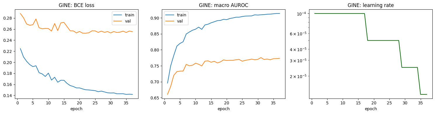
plot_diagnostics(gine_history, "GINE")

As we can see, there is a clear gap between the training and validation loss, indicating that the model is overfitting. In the future, a hyperparameter sweep can be performed to find the optimal model architecture and training parameters to reduce overfitting.

# Evaluate on test data
gine_test_loss, gine_test_macro, gine_test_per_task, gine_test_proba = evaluate_gine(
    gine_model, test_loader, TOX21_TASKS
)
print("GINE — test macro:\n", gine_test_macro)

Output:

GINE — test macro:
 auroc    0.752415
auprc    0.367339
bce      0.268268
dtype: float64

print(gine_test_per_task)

Output:

               n_not_missing     auroc     auprc       bce
task                                                      
NR-AR                    710  0.756275  0.410758  0.139618
NR-AR-LBD                625  0.784992  0.430528  0.121509
NR-AhR                   631  0.861561  0.611699  0.289744
NR-Aromatase             513  0.759482  0.408706  0.281288
NR-ER                    542  0.711959  0.429774  0.369044
NR-ER-LBD                654  0.722159  0.337079  0.155390
NR-PPAR-gamma            573  0.710114  0.096841  0.160126
SR-ARE                   461  0.737652  0.468324  0.535995
SR-ATAD5                 666  0.710179  0.204821  0.204716
SR-HSE                   564  0.735774  0.234789  0.255386
SR-MMP                   517  0.828037  0.547383  0.373727
SR-p53                   633  0.710802  0.227364  0.332671

Model 3: Chemprop

Chemprop data workflow:

• Create Mol objects and RDKit 2D features (x_d): make_rdkit2d_features.
• Create MoleculeDatapoint objects: for each molecule, combine its Mol object, labels (y), and any extra features (x_d) into a MoleculeDatapoint instance (via make_datapoints).
• Create MoleculeDataset objects: collect these MoleculeDatapoint instances into MoleculeDatasets for the train, validation, and test sets. Provide a graph featurizer to the dataset.
• Create DataLoaders: pass these MoleculeDataset objects to build_dataloader to create iterable loaders that feed batches of graph data to the Chemprop model during training and evaluation.

Extracting features

During my initial training, I noticed that the Chemprop model was producing astronomical loss values. Upon investigation, I found that some of the 2D features had extreme values (likely Ipc/Kappa3, similarly reported here) that had corrupted the training steps. The short-term solution is to clip these values to \(1e^6\) to prevent them from blowing up the scaling and downstream logits/loss to nonsensical magnitudes.

def make_rdkit2d_features(
    smiles_list: list[str],
    clip_max: float = 1e6,
) -> tuple[list, np.ndarray]:
    """
    Compute chemprop's RDKit 2D descriptors, guarding against known-pathological
    descriptors (notably Ipc, and occasionally Kappa3) that can return finite-but-
    astronomically-large values (documented up to ~1e162 for Ipc on real molecules,
    see rdkit/rdkit#1527) for some molecules. These pass straight through
    nan_to_num(posinf=...) since they aren't literally inf, but blow up scaling and
    downstream logits/loss to nonsensical magnitudes. Hard-clipping is a blunt but
    reliable guard against any similarly-behaved descriptor, not just Ipc specifically.
    """
    mol_featurizer = cp_featurizers.MoleculeFeaturizerRegistry["rdkit_2d"]()
    mols = [cp_utils.make_mol(smi, keep_h=False, add_h=False) for smi in smiles_list]
    X_d = np.array([mol_featurizer(m) for m in mols], dtype=np.float64)
    X_d = np.nan_to_num(X_d, nan=0.0, posinf=0.0, neginf=0.0)

    n_clipped = int(np.sum(np.abs(X_d) > clip_max))
    if n_clipped:
        print(f"clipping {n_clipped} extreme RDKit 2D feature values (|x| > {clip_max:.0e}), likely Ipc/Kappa3")
    X_d = np.clip(X_d, -clip_max, clip_max).astype(np.float32)
    return mols, X_d

def make_datapoints(
    smiles_list: list[str],
    y_arr: np.ndarray,
    w_arr: np.ndarray,
    mols: list,
    X_d: np.ndarray,
) -> list:
    """
    Build chemprop MoleculeDatapoints, masking missing labels as NaN.

    Raises if any SMILES failed to parse via cp_utils.make_mol (mols contains None),
    since that would otherwise fail silently or misalign rows downstream.
    """
    none_idx = [i for i, m in enumerate(mols) if m is None]
    if none_idx:
        raise ValueError(f"{len(none_idx)} SMILES failed chemprop parsing, e.g. {smiles_list[none_idx[0]]!r}")
    assert len(smiles_list) == len(y_arr) == len(w_arr) == len(mols) == len(X_d), "length mismatch"

    y_masked = y_arr.copy()
    y_masked[w_arr <= 0] = np.nan
    return [
        cp_data.MoleculeDatapoint(mol, y, x_d=xd)
        for mol, y, xd in zip(mols, y_masked, X_d)
    ]

train_mols, X_d_train = make_rdkit2d_features(train_smiles)
val_mols,   X_d_val   = make_rdkit2d_features(val_smiles)
test_mols,  X_d_test  = make_rdkit2d_features(test_smiles)

cp_train_data = make_datapoints(train_smiles, y_train, w_train, train_mols, X_d_train)
cp_val_data   = make_datapoints(val_smiles,   y_val,   w_val,   val_mols,   X_d_val)
cp_test_data  = make_datapoints(test_smiles,  y_test,  w_test,  test_mols,  X_d_test)

print("RDKit 2D feature dim:", X_d_train.shape[1])

# The featurizer convert Mol to graph attributes e.g. nodes, edges, attributes
molgraph_featurizer = cp_featurizers.SimpleMoleculeMolGraphFeaturizer()

cp_train_dset = cp_data.MoleculeDataset(cp_train_data, molgraph_featurizer)
cp_val_dset   = cp_data.MoleculeDataset(cp_val_data,   molgraph_featurizer)
cp_test_dset  = cp_data.MoleculeDataset(cp_test_data,  molgraph_featurizer)

Output:

WARNING:chemprop.featurizers.molecule:The RDKit 2D features can deviate signifcantly from a normal distribution. Consider manually scaling them using an appropriate scaler before creating datapoints, rather than using the scikit-learn `StandardScaler` (the default in Chemprop).

clipping 321 extreme RDKit 2D feature values (|x| > 1e+06), likely Ipc/Kappa3

RDKit 2D feature dim: 217

As we can see from the output, the RDKit 2D features can deviate significantly from a normal distribution. Therefore, we will use a robust scaler (median & IQR scaling) to scale the features instead of the default StandardScaler in Chemprop.

Scaling features

# Scale 2D descriptors with robust scaler (scale with median, IQR)
from sklearn.preprocessing import RobustScaler, StandardScaler

def make_robust_x_d_scaler(X_d_train: np.ndarray) -> StandardScaler:
    """
    Fit sklearn's RobustScaler (median/IQR) on raw extra features, then repackage
    its fitted stats into a StandardScaler-shaped object.

    chemprop's normalize_inputs() / ScaleTransform.from_standard_scaler() are typed
    specifically to StandardScaler and read its .mean_/.scale_ attributes at transform
    time — a raw RobustScaler (.center_/.scale_) isn't a drop-in replacement. Building
    a genuine StandardScaler instance and overwriting its fitted attributes keeps any
    isinstance checks happy while making .transform() behave like RobustScaler
    (median-centered, IQR-scaled) instead of mean/std-based scaling.

    RobustScaler is generally more appropriate here than StandardScaler, since RDKit 2D
    descriptors (MolWt, ring counts, etc.) are known to deviate significantly from a
    normal distribution and can have long-tailed outliers that StandardScaler is
    sensitive to but median/IQR scaling is not.
    """
    robust = RobustScaler()
    robust.fit(X_d_train)

    x_d_scaler = StandardScaler()
    x_d_scaler.mean_ = robust.center_                                   # median per feature
    x_d_scaler.scale_ = np.where(robust.scale_ == 0, 1.0, robust.scale_)  # IQR per feature, guarded against div-by-zero
    x_d_scaler.var_ = x_d_scaler.scale_ ** 2                             # kept consistent in case anything reads var_
    x_d_scaler.n_features_in_ = X_d_train.shape[1]
    return x_d_scaler

# Fit once on train, apply (not re-fit) to all three splits — same pattern as the
# original StandardScaler-based code, just swap the fitting step:
x_d_scaler = make_robust_x_d_scaler(X_d_train)

cp_train_dset.normalize_inputs("X_d", x_d_scaler)
cp_val_dset.normalize_inputs("X_d", x_d_scaler)
cp_test_dset.normalize_inputs("X_d", x_d_scaler)

# Cache processed graph representations to speed up subsequent epochs
cp_train_dset.cache = True
cp_val_dset.cache = True

BATCH_SIZE_CP = 50  # matches the Chemprop v1/v2 literature default
cp_train_loader = cp_data.build_dataloader(cp_train_dset, batch_size=BATCH_SIZE_CP, num_workers=0)
cp_val_loader   = cp_data.build_dataloader(cp_val_dset,   batch_size=BATCH_SIZE_CP, num_workers=0, shuffle=False)
cp_test_loader  = cp_data.build_dataloader(cp_test_dset,  batch_size=BATCH_SIZE_CP, num_workers=0, shuffle=False)

Chemprop model

Let’s build the Chemprop model. The Chemprop model consists of three main components: D-MPNN message-passing module, a graph-level aggregation module, and a feedforward neural network (FFN) for binary classification.

HIDDEN_DIM = 128
DEPTH = 3
DROPOUT = 0.2

mp = cp_nn.BondMessagePassing(
    d_h=HIDDEN_DIM, depth=DEPTH, dropout=DROPOUT,
)
agg = cp_nn.MeanAggregation()

ffn_input_dim = mp.output_dim + X_d_train.shape[1]
ffn = cp_nn.BinaryClassificationFFN(
    n_tasks=N_TASKS, input_dim=ffn_input_dim, hidden_dim=HIDDEN_DIM,
    n_layers=2, dropout=DROPOUT,
)

X_d_transform = cp_nn.ScaleTransform.from_standard_scaler(x_d_scaler)

metric_list = [cp_nn.metrics.BinaryAUROC(), cp_nn.metrics.BinaryAUPRC()]

chemprop_model = cp_models.MPNN(
    mp, agg, ffn, batch_norm=True, metrics=metric_list,
    X_d_transform=X_d_transform,
    warmup_epochs=2, init_lr=1e-4, max_lr=1e-3, final_lr=1e-5,
)
print(chemprop_model)

Output:

MPNN(
  (message_passing): BondMessagePassing(
    (W_i): Linear(in_features=86, out_features=128, bias=False)
    (W_h): Linear(in_features=128, out_features=128, bias=False)
    (W_o): Linear(in_features=200, out_features=128, bias=True)
    (dropout): Dropout(p=0.2, inplace=False)
    (tau): ReLU()
    (V_d_transform): Identity()
    (graph_transform): Identity()
  )
  (agg): MeanAggregation()
  (bn): BatchNorm1d(128, eps=1e-05, momentum=0.1, affine=True, track_running_stats=True)
  (predictor): BinaryClassificationFFN(
    (ffn): MLP(
      (0): Sequential(
        (0): Linear(in_features=345, out_features=128, bias=True)
      )
      (1): Sequential(
        (0): ReLU()
        (1): Dropout(p=0.2, inplace=False)
        (2): Linear(in_features=128, out_features=128, bias=True)
      )
      (2): Sequential(
        (0): ReLU()
        (1): Dropout(p=0.2, inplace=False)
        (2): Linear(in_features=128, out_features=12, bias=True)
      )
    )
    (criterion): BCELoss(task_weights=[[1.0, 1.0, 1.0, 1.0, 1.0, 1.0, 1.0, 1.0, 1.0, 1.0, 1.0, 1.0]])
    (output_transform): Identity()
  )
  (X_d_transform): ScaleTransform()
  (metrics): ModuleList(
    (0): BinaryAUROC()
    (1): BinaryAUPRC()
    (2): BCELoss(task_weights=[[1.0, 1.0, 1.0, 1.0, 1.0, 1.0, 1.0, 1.0, 1.0, 1.0, 1.0, 1.0]])
  )
)

Note that Chemprop uses its own internal atom/bond featurization via SimpleMoleculeMolGraphFeaturizer — separate from, and a different dimensionality than, the custom 52/10-dim atom/bond features hand-built for GINE above. This is visible in the model summary’s W_i: Linear(in_features=86, ...) layer, which reflects Chemprop’s own atom+bond feature concatenation width, not the 52/10 dims computed earlier for GINE.

Training

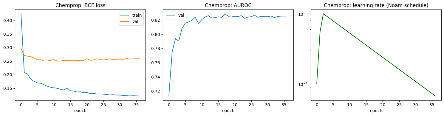
Similar to the GINE model, we will use early stopping and learning rate scheduling to prevent overfitting. The Chemprop model will be trained for a maximum of 60 epochs, with early stopping patience of 25 epochs. The best model will be saved to the /chemprop directory.

import os
save_path = "/chemprop"
os.makedirs(save_path, exist_ok=True)
logger = CSVLogger(save_path, name="tox21_chemprop")
checkpoint_cb = ModelCheckpoint(
    save_path, "best-{epoch}-{val_loss:.3f}", monitor="val_loss", mode="min", save_last=True,
)
early_stop_cb = EarlyStopping(monitor="val_loss", mode="min", patience=25)
lr_monitor_cb = LearningRateMonitor(logging_interval="epoch")

trainer = pl.Trainer(
    logger=logger,
    enable_checkpointing=True,
    enable_progress_bar=True,
    accelerator="auto", # auto select cpu or gpu
    devices=1, # how many cores
    max_epochs=60,
    callbacks=[checkpoint_cb, early_stop_cb, lr_monitor_cb],
)

trainer.fit(chemprop_model, cp_train_loader, cp_val_loader)

Output:

┏━━━┳━━━━━━━━━━━━━━━━━┳━━━━━━━━━━━━━━━━━━━━━━━━━┳━━━━━━━━┳━━━━━━━┳━━━━━━━┓
┃   ┃ Name            ┃ Type                    ┃ Params ┃ Mode  ┃ FLOPs ┃
┡━━━╇━━━━━━━━━━━━━━━━━╇━━━━━━━━━━━━━━━━━━━━━━━━━╇━━━━━━━━╇━━━━━━━╇━━━━━━━┩
│ 0 │ message_passing │ BondMessagePassing      │ 53.1 K │ train │     0 │
│ 1 │ agg             │ MeanAggregation         │      0 │ train │     0 │
│ 2 │ bn              │ BatchNorm1d             │    256 │ train │     0 │
│ 3 │ predictor       │ BinaryClassificationFFN │ 62.3 K │ train │     0 │
│ 4 │ X_d_transform   │ ScaleTransform          │      0 │ train │     0 │
│ 5 │ metrics         │ ModuleList              │      0 │ train │     0 │
└───┴─────────────────┴─────────────────────────┴────────┴───────┴───────┘

Trainable params: 115 K                                                                                            
Non-trainable params: 0                                                                                            
Total params: 115 K                                                                                                
Total estimated model params size (MB): 0.463                                                                      
Modules in train mode: 27                                                                                          
Modules in eval mode: 0                                                                                            
Total FLOPs: 0                                                                                                     

Epoch 36/59 ━━━━━━━━━━━━━━━━━━━━━━━━━━━━━━━━ 126/126 0:00:02 • 0:00:00 46.86it/s v_num: 2.000 train_loss_step:     
                                                                                 0.262 val_loss: 0.259             
                                                                                 train_loss_epoch: 0.121           

Evaluation

# Pull per-epoch metrics back out of the CSV logger for diagnostic plots
metrics_path = f"{logger.log_dir}/metrics.csv"
cp_metrics_df = pd.read_csv(metrics_path)

def epoch_series(df: pd.DataFrame, col: str) -> pd.Series:
    """
    Extract a per-epoch series from chemprop's CSVLogger metrics.csv.

    LearningRateMonitor logs LR rows with a blank `epoch` (keyed by step instead),
    so back-fill epoch from the next non-null row before dropping NaNs, rather than
    dropping rows that only lack an epoch stamp but do have a valid value.
    """
    sub = df[["epoch", col]].copy()
    sub["epoch"] = sub["epoch"].bfill()
    sub = sub.dropna(subset=[col])
    return sub.groupby("epoch")[col].mean()

cp_history = {
    "train_loss": epoch_series(cp_metrics_df, "train_loss_epoch") if "train_loss_epoch" in cp_metrics_df else epoch_series(cp_metrics_df, "train_loss"),
    "val_loss": epoch_series(cp_metrics_df, "val_loss"),
    "lr": epoch_series(cp_metrics_df, [c for c in cp_metrics_df.columns if c.startswith("lr-")][0]),
}
# AUROC column names in chemprop v2's metric logging follow "val/roc"-style keys; adjust if your version differs
auroc_col_candidates = [c for c in cp_metrics_df.columns if "roc" in c.lower() and "val" in c.lower()]
train_auroc_candidates = [c for c in cp_metrics_df.columns if "roc" in c.lower() and "train" in c.lower()]
if auroc_col_candidates:
    cp_history["val_auroc"] = epoch_series(cp_metrics_df, auroc_col_candidates[0])
if train_auroc_candidates:
    cp_history["train_auroc"] = epoch_series(cp_metrics_df, train_auroc_candidates[0])

fig, axes = plt.subplots(1, 3, figsize=(15, 4))

axes[0].plot(cp_history["train_loss"].index, cp_history["train_loss"].values, label="train")
axes[0].plot(cp_history["val_loss"].index, cp_history["val_loss"].values, label="val")
axes[0].set_title("Chemprop: BCE loss"); axes[0].set_xlabel("epoch"); axes[0].legend()

if "val_auroc" in cp_history:
    if "train_auroc" in cp_history:
        axes[1].plot(cp_history["train_auroc"].index, cp_history["train_auroc"].values, label="train")
    axes[1].plot(cp_history["val_auroc"].index, cp_history["val_auroc"].values, label="val")
    axes[1].set_title("Chemprop: AUROC"); axes[1].set_xlabel("epoch"); axes[1].legend()
else:
    axes[1].set_title("AUROC column not found in metrics.csv — see printed columns above")

axes[2].plot(cp_history["lr"].index, cp_history["lr"].values, color="darkgreen")
axes[2].set_title("Chemprop: learning rate (Noam schedule)"); axes[2].set_xlabel("epoch"); axes[2].set_yscale("log")

plt.tight_layout()
plt.show()

We can see here that the Chemprop model is overfitting, as the training loss continues to decrease while the validation loss stays flat. A few things to bring up:

• The RDKit 2D feature clipping may not be the best fix. Clipping the Ipc/Kappa3 descriptor values to ±1e6 stops the numerical blow-up, but the clipped values themselves are still a somewhat arbitrary cutoff rather than a well-scaled feature — a log-transform of Ipc specifically (or dropping it entirely) would probably be a good fix.
• The learning rate schedule likely hadn’t finished annealing when early stopping fired. Chemprop’s Noam scheduler decay length is computed from trainer.max_epochs (60 here), not from whichever epoch early stopping actually lands on — so the LR at the “best” checkpoint may still be well above the intended final_lr.
• Chemprop defaults to plain Adam with no weight decay option on the public API — unlike the GINE loop above, which explicitly sets weight_decay in AdamW. There are ways to incorporate wieght decay into the workflow but will not be discussed here.

# Per-task metrics, computed the same way as RF/GINE for a like-for-like comparison table
chemprop_model.eval()
with torch.no_grad():
    preds = trainer.predict(chemprop_model, cp_test_loader, ckpt_path="best", weights_only=False)
    cp_test_proba = torch.cat(preds, dim=0).numpy()

cp_test_per_task, cp_test_macro = masked_task_metrics(y_test, cp_test_proba, w_test, TOX21_TASKS)
print("Chemprop — test macro:\n", cp_test_macro)

Output:

Chemprop — test macro:
 auroc    0.714631
auprc    0.264956
bce      0.410267
dtype: float64

print(cp_test_per_task)

Output:

               n_not_missing     auroc     auprc       bce
task                                                      
NR-AR                    710  0.674216  0.290272  0.257757
NR-AR-LBD                625  0.834176  0.252088  0.157581
NR-AhR                   631  0.763444  0.405000  0.581689
NR-Aromatase             513  0.694687  0.229284  0.614416
NR-ER                    542  0.652002  0.276363  0.569813
NR-ER-LBD                654  0.747490  0.187147  0.185182
NR-PPAR-gamma            573  0.621597  0.076866  0.236523
SR-ARE                   461  0.711489  0.464259  0.628591
SR-ATAD5                 666  0.634082  0.105101  0.310851
SR-HSE                   564  0.738257  0.205279  0.278903
SR-MMP                   517  0.795859  0.441507  0.668769
SR-p53                   633  0.708277  0.246308  0.433123

Model comparison

comparison = pd.DataFrame({
    "RF + ECFP2048": rf_test_macro,
    "GINE": gine_test_macro,
    "Chemprop (+ RDKit2D)": cp_test_macro,
}).T
print(comparison)

Output:

                         auroc     auprc       bce
RF + ECFP2048         0.732228  0.382328  0.287920
GINE                  0.752415  0.367339  0.268268
Chemprop (+ RDKit2D)  0.714631  0.264956  0.410267

fig, ax = plt.subplots(figsize=(7, 4))
comparison[["auroc", "auprc"]].plot.bar(ax=ax)
ax.set_ylabel("macro score (test set)")
ax.set_title("Test-set macro AUROC / AUPRC by model")
ax.set_ylim(0, 1)
plt.xticks(rotation=15)
plt.tight_layout()
plt.show()

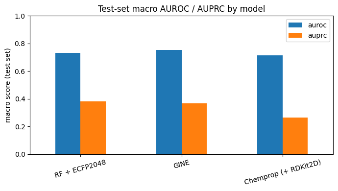
As we can see from the comparison table and bar plot, RF and GINE have quite similar performance on the test set, with GINE having the best performance in terms of AUROC and BCE loss, while RF + ECFP2048 has the best AUPRC. Chemprop’s AUPRC (0.265) sits below both (0.37-0.38) — potentially due to the contributing factors discussed above. Again, the RF model is well-tuned while the GINE and Chemprop models are trained with pre-selected hyperparameters, so further fine-tuning can be performed to improve their performance. In addition, deep learning models typically require larger datasets (e.g. >10k) to learn meaningful patterns from the data. The Tox21 data, with ~7,800 data points, is on the smaller side for a flexible GNN to fine-tune its parameters. Thus, in which case that the available dataset is small, a classical ML approach is likely the better choice for prediction.

t-SNE of the learned representations

The question here is that: do the learned graph representations (embeddings) from GINE and Chemprop models capture some chemical information that can be visualized in a low-dimensional space? To answer that, we will use t-SNE to reduce the dimensionality of the learned embeddings to 2D and visualize them with different overlays (molecular properties such as molecular weight, LogP and TPSA, and 2 task labels).

Extracting the GINE learned graph representations (embeddings) from the test set:

@torch.no_grad()
def extract_gine_embeddings(model, loader):
    model.eval()
    embs, smiles_list = [], []
    for batch in loader:
        batch = batch.to(DEVICE)
        emb = model.embed(batch.x, batch.edge_index, batch.edge_attr, batch.batch)
        embs.append(emb.cpu().numpy()) # [(B, 256), (B, 256), ...]
        smiles_list.extend(batch.smiles)
    return np.concatenate(embs, axis=0), smiles_list # concat embs on rows: (N, 256)

gine_test_embeddings, gine_test_smiles_order = extract_gine_embeddings(gine_model, test_loader) # (N, 256)
print("GINE test embedding matrix:", gine_test_embeddings.shape)

Output:

GINE test embedding matrix: (783, 256)

Extracting the Chemprop learned graph representations (embeddings) from the test set:

@torch.no_grad()
def extract_chemprop_embeddings(model, loader):
    model.eval()
    embs = []
    for batch in loader:
        emb = model.encoding(batch.bmg, batch.V_d, batch.X_d, i=0)
        # batch.bmg: BatchMolGraph - batch disjoint graph
        # batch.V_d: atom features
        # batch.X_d: 2D descriptors
        # i=0: extract embed right before FFN
        embs.append(emb.cpu().numpy())
    return np.concatenate(embs, axis=0) # (N, HIDDEN_DIM + X_d_train.shape[1])

chemprop_test_embeddings = extract_chemprop_embeddings(chemprop_model, cp_test_loader)
print("Chemprop test embedding matrix:", chemprop_test_embeddings.shape)

Output:

Chemprop test embedding matrix: (783, 345)

Computing some molecular properties and task labels for coloring the t-SNE plots. The properties are computed using RDKit’s Descriptors and Crippen modules, while the task labels are extracted from the test set labels and weights.

def compute_property(smiles_list, fn):
    vals = np.full(len(smiles_list), np.nan)
    for i, smi in enumerate(smiles_list):
        mol = Chem.MolFromSmiles(smi)
        if mol is not None:
            vals[i] = fn(mol)
    return vals

# gine_test_smiles_order is the exact row order of gine_test_embeddings (PyG loader order,
# with unparseable SMILES already dropped) — properties/labels must be looked up in that order.
mol_wt   = compute_property(gine_test_smiles_order, Descriptors.MolWt)
logp     = compute_property(gine_test_smiles_order, Crippen.MolLogP)
tpsa     = compute_property(gine_test_smiles_order, Descriptors.TPSA)

smi_to_idx = {s: i for i, s in enumerate(test_smiles)}
order_idx = np.array([smi_to_idx[s] for s in gine_test_smiles_order])
nr_ar  = np.where(w_test[order_idx, TOX21_TASKS.index("NR-AR")] > 0,
                   y_test[order_idx, TOX21_TASKS.index("NR-AR")], np.nan)
sr_mmp = np.where(w_test[order_idx, TOX21_TASKS.index("SR-MMP")] > 0,
                   y_test[order_idx, TOX21_TASKS.index("SR-MMP")], np.nan)
                   
def tsne_embed(X, seed=SEED):
    return TSNE(n_components=2, perplexity=30, init="pca", random_state=seed).fit_transform(X)

gine_tsne = tsne_embed(gine_test_embeddings)
# Chemprop's test loader order matches cp_test_data / test_smiles directly (no drops, since
# chemprop's utils.make_mol handles the same SMILES successfully parsed earlier by RDKit)
chemprop_tsne = tsne_embed(chemprop_test_embeddings)

Plotting the t-SNE embeddings with different overlays (molecular properties and task labels) for both GINE and Chemprop models:

def plot_tsne_grid(tsne_xy, overlays, model_name):
    fig, axes = plt.subplots(1, len(overlays), figsize=(5 * len(overlays), 4.5))
    for ax, (label, values, cmap, discrete) in zip(axes, overlays):
        nan_mask = np.isnan(values)
        ax.scatter(tsne_xy[nan_mask, 0], tsne_xy[nan_mask, 1], c="lightgrey", s=10, label="missing")
        sc = ax.scatter(tsne_xy[~nan_mask, 0], tsne_xy[~nan_mask, 1],
                         c=values[~nan_mask], cmap=cmap, s=12,
                         vmin=0 if discrete else None, vmax=1 if discrete else None)
        plt.colorbar(sc, ax=ax, fraction=0.046)
        ax.set_title(f"{model_name}: colored by {label}")
        ax.set_xticks([]); ax.set_yticks([])
    plt.tight_layout()
    plt.show()

overlays = [
    ("MolWt", mol_wt, "viridis", False),
    ("LogP", logp, "viridis", False),
    ("TPSA", tpsa, "viridis", False),
    ("NR-AR (active=1)", nr_ar, "coolwarm", True),
    ("SR-MMP (active=1)", sr_mmp, "coolwarm", True),
]

plot_tsne_grid(gine_tsne, overlays, "GINE")

plot_tsne_grid(chemprop_tsne, overlays, "Chemprop")

As we can see, the t-SNE embeddings from both GINE and Chemprop models show mild clustering patterns based on molecular properties and task labels, suggesting that the learned graph representations capture some chemical information. Further analysis and interpretation (e.g. tune t-SNE perplexity, or try UMAP) of these embeddings can be performed to understand the relationships between molecular structures and their properties.

Disclosures

The code was written with the aid of Claude Sonnet 5, and the model training was performed on Google Colab Pro+ with a Tesla T4 GPU. The accuracy of the code was verified by the author.

References

• Yang, K. et al. “Analyzing Learned Molecular Representations for Property Prediction.” J. Chem. Inf. Model. 2019, 59, 8, 3370–3388.
• Heid, E. et al. “Chemprop: A Machine Learning Package for Chemical Property Prediction.” J. Chem. Inf. Model. 2024, 64, 1, 9–17.
• Xu, K. et al. “How Powerful are Graph Neural Networks?” ICLR 2019. (GIN)
• Hu, W. et al. “Strategies for Pre-training Graph Neural Networks.” ICLR 2020. (GINE’s edge-feature extension)
• Wu, Z. et al. “MoleculeNet: A Benchmark for Molecular Machine Learning.” Chem. Sci. 2018, 9, 513–530.
• Bemis, G.W.; Murcko, M.A. “The Properties of Known Drugs. 1. Molecular Frameworks.” J. Med. Chem. 1996, 39, 15, 2887–2893. (Bemis-Murcko scaffolds)
• Huang, R. et al. “Tox21 Challenge to Build Predictive Models of Nuclear Receptor and Stress Response Pathways as Mediated by Exposure to Environmental Chemicals and Drugs.” Front. Environ. Sci. 2016.
• TeachOpenCADD GNN tutorial (T035)
• RDKit Ipc descriptor overflow, GitHub issue #1527