Code
all_dat['train'].head()To accurately predict peptide-MHCII binding affinity, I developed a 1D Convolutional Neural Network (CNN) combined with Multi-Layer Perceptron (MLP) model using protein embeddings from the ESM2 large language model.
Comparing with a simpler MLP-only model, the CNN + MLP model demonstrated over 12% improvement in peptide-MHCII binding prediction accuracy, achieving an \(R^2\) score of 0.62 for all MHC alleles, and close to 0.8 for specific alleles. Saliency Map and In Silico Mutagenesis analyses revealed key amino acid positions that significantly influence binding affinity predictions, providing insights into the underlying biological interactions.
This exercise showcases the potential of combining Large Language Models with machine learning to tackle complex biological challenges. These could range from predicting protein-protein interactions and drug-target binding to forecasting drug responses from gene expression data.
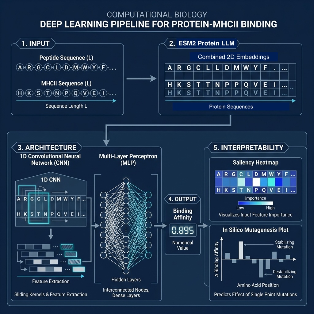
In my last post, I explored the use of protein large language model (LLM) embeddings from ESM2 for predicting peptide-MHCII binding affinity using a Multi-Layer Perceptron (MLP). While the MLP performed reasonably well, I believe that incorporating Convolutional Neural Networks (CNNs) could further enhance the model’s ability to capture local sequence patterns in the protein embeddings.
The protein sequence embeddings generated by ESM2 are typically 2-dimensional arrays, where one dimension represents the amino acid sequence and the other represents the embedding features. In my previous approach, I flattened these embeddings into 1-dimensional vectors by taking the mean before feeding them into the MLP. However, this flattening process may lead to the loss of important spatial relationships between amino acids in the sequence.
In this post, I will implement a 1D CNN to process the full embeddings from ESM2 without pre-flattening. I will apply 2 layers of 1D convolution followed by average pooling to capture local patterns in the sequence embeddings. After the CNN layers, I will add fully connected MLP layers to perform the final prediction task. I will compare the performance of this CNN + MLP model with a similar MLP-only model to evaluate the impact of incorporating convolutional layers.
Finally, to understand which amino acid positions contribute most to the binding affinity predictions, I will perform Saliency Map analysis on both the peptide and MHCII sequences, using gradients calculated from the model outputs with respect to the input embeddings. I will also perform an In Silico Mutagenesis (ISM) analysis to see how disruptive single amino acid changes affect the predicted binding affinity.
I will not go through all the steps in detail, as they are similar to my previous post. Instead, I will highlight the key steps involved in this approach:
Embeddings Extraction: We will have to modify the embeddings extraction code to retain the 2D structure of the embeddings. We need to input the max sequence length to ensure consistent input sizes for the model. After that, we will concatenate the peptide and MHC2 embeddings along the sequence length dimension, retaining the sequence information and the 2D structure. This allows for the saliency map analysis later on.
Model Architecture: We will define a new model architecture that includes 1D convolutional layers followed by dense layers. Using the functional API in TensorFlow/Keras, we will create a model that takes the 2D embeddings and peptide/MHC sequence lengths as inputs, applies convolutional layers, and then concatenates them to pass it through dense layers to make the final prediction.
Training and Evaluation: We will train the new model and evaluate its performance against a similar MLP-only model, to see if the CNN layers improve binding affinity prediction.
Saliency Map and In Silico Mutagenesis Analysis: We will compute saliency maps to identify important amino acid positions in the peptide and MHC2 sequences that influence binding affinity predictions. We will also perform ISM to assess the impact of single amino acid mutations on the predicted affinity.
First, let’s see what the input data looks like:
all_dat['train'].head()Output:
   Peptide_ID           Peptide     MHC_ID  \
0      104653   VAPIEHIASMRRNYF  DRB1_1302
1       37106   HDDKETSFIRNCARK  DRB1_0101
2      118433   LIWVGINTRNMTMSM  DRB1_0101
3       80770  GVTVIKNNMINNDLGP  DRB1_1501
4       19888   PAPMLAAAAGWQTLS  DRB1_1101

                                  MHC         Y
0  QEFFIASGAAVDAIMESSFDYFDIDEATYHVGFT  0.501084
1  QEFFIASGAAVDAIMWLFLECYDLQRATYHVGFT  0.441298
2  QEFFIASGAAVDAIMWLFLECYDLQRATYHVGFT  0.217673
3  QEFFIASGAAVDAIMWPRFDYFDIQAATYHVVFT  0.807811
4  QEFFIASGAAVDAIMESSFDYFDFDRATYHVGFT  0.583271
all_dat is a dictionary containing the training, validation, and test datasets as dataframes, each with peptide and MHC2 sequences, and binding affinity Y.
The embeddings extraction code to retain the 2D structure of the embeddings:
from transformers import AutoTokenizer, EsmModel
import numpy as np
import torch
import math
from tqdm import tqdm

# Load pre-trained ESM2 model and tokenizer
model_checkpoint = "facebook/esm2_t30_150M_UR50D" # 640 dim
tokenizer = AutoTokenizer.from_pretrained(model_checkpoint)
model = EsmModel.from_pretrained(model_checkpoint)

# Function to get embeddings
def extract_full_embedding(
    sequence: list[str],
    tokenizer: AutoTokenizer,
    model: EsmModel,
    device: torch.device | None = None,
    batch_size: int = 64,
    max_len: int = 50
    ) -> np.ndarray:

    """Extract full embeddings for peptide sequences from an LLM model.
       Batch iteration is required as this is memory intensive."""

    # Use GPU when available
    if not device:
        device = torch.device("cuda" if torch.cuda.is_available() else "cpu")

    # Separate sequence list into batches
    n_batches = math.ceil(len(sequence) / batch_size)
    all_batch_embeddings = []

    model = model.to(device) # Move model to the target device
    model.eval() # Set model to evaluation mode

    steps = tqdm(range(n_batches))

    for i in steps:
        steps.set_description(f"Processing batch {i+1}/{n_batches}")
        start = i * batch_size
        end = (i + 1) * batch_size
        batch = sequence[start:end]

        # Tokenize peptide sequence and pad to max length
        inputs = tokenizer(batch, return_tensors="pt", padding='max_length', truncation=True, max_length=max_len)

        # Move input to the target device
        inputs = {name: tensor.to(device) for name, tensor in inputs.items()}

        # Forward pass through the model without gradient tracking to get embeddings
        with torch.no_grad():
          batch_mean_embeddings = model(**inputs).last_hidden_state.detach().cpu().numpy()
        all_batch_embeddings.append(batch_mean_embeddings)

    embeddings = np.concatenate(all_batch_embeddings, axis=0)
    # This will return a (N_samples, max_len, n_dim) array
    return embeddings
Since each peptide and MHC2 sequence can have different lengths, we need to pad them to a consistent length during the embedding extraction so that they can be concatenated later. Let’s get the max sequence lengths for peptides or MHC2 sequences so we can pad the embeddings accordingly.
length_pt = []
for df in all_dat.values():
  length_pt.append(df['Peptide'].apply(len).max())
max_len_pt = max(length_pt)

length_mhc = []
for df in all_dat.values():
  length_mhc.append(df['MHC'].apply(len).max())
max_len_mhc = max(length_mhc)

print(max_len_pt, max_len_mhc)
Output:
37 34The maximum peptide length is 37, and the maximum MHC2 length is 34.
Now we can extract the full embeddings for both peptides and MHC2 sequences, and pad them each to their respective max lengths.
embedding_dict_pt = {}
for data, sequence in sequence_dict_pt.items():
    print(f"Extracting embeddings for {data}...")
    embedding_dict_pt[data] = extract_full_embedding(sequence, tokenizer, model, batch_size=1280, max_len=max_len_pt)

embedding_dict_mhc = {}
for data, sequence in sequence_dict_mhc.items():
    print(f"Extracting embeddings for {data}...")
    embedding_dict_mhc[data] = extract_full_embedding(sequence, tokenizer, model, batch_size=1280, max_len=max_len_mhc)
Concatenate the peptide and MHC2 embeddings along the sequence dimension (axis=1) to create the final input embeddings for our model.
embedding_dict = {}
for data_type in ['train', 'valid', 'test']:
  pt_embeddings = embedding_dict_pt[f'{data_type}_pt']
  mhc_embeddings = embedding_dict_mhc[f'{data_type}_mhc']
  # Concatenate along the sequence length axis
  embedding_dict[data_type] = np.concatenate([pt_embeddings, mhc_embeddings], axis=1)

# Print shapes to verify
for key, value in embedding_dict.items():
  print(f"Shape of {key} combined embeddings: {value.shape}")
Output:
Shape of train combined embeddings: (82388, 71, 640)
Shape of valid combined embeddings: (11702, 71, 640)
Shape of test combined embeddings: (23410, 71, 640)
The output here is: (sample size, sequence_length, embedding_dimension).
Finally, we need to determine the actual lengths of each peptide and MHC2 sequence (before padding) to provide as additional inputs to the model:
# Determine each peptide or MHC sequence length to add into the embeddings for training input
seq_length_pt = {}
for key, sequence in sequence_dict_pt.items():
    seq_length_pt[key] = [len(seq) for seq in sequence]

seq_length_mhc = {}
for key, sequence in sequence_dict_mhc.items():
seq_length_mhc[key] = [len(seq) for seq in sequence]Make the TensorFlow datasets from these 2D embeddings.
# Convert data to Tensorflow dataset
import tensorflow as tf

# Embeddings (already concatenated along sequence length axis)
X_train_emb = embedding_dict['train']
X_valid_emb = embedding_dict['valid']
X_test_emb = embedding_dict['test']

# Target variable
y_train = all_dat['train']['Y'].values
y_valid = all_dat['valid']['Y'].values
y_test = all_dat['test']['Y'].values

# Sequence lengths (converting lists to numpy arrays and then to tf tensors)
X_train_pt_len = tf.convert_to_tensor(np.array(seq_length_pt['train_pt']), dtype=tf.float32)
X_train_mhc_len = tf.convert_to_tensor(np.array(seq_length_mhc['train_mhc']), dtype=tf.float32)
X_valid_pt_len = tf.convert_to_tensor(np.array(seq_length_pt['valid_pt']), dtype=tf.float32)
X_valid_mhc_len = tf.convert_to_tensor(np.array(seq_length_mhc['valid_mhc']), dtype=tf.float32)
X_test_pt_len = tf.convert_to_tensor(np.array(seq_length_pt['test_pt']), dtype=tf.float32)
X_test_mhc_len = tf.convert_to_tensor(np.array(seq_length_mhc['test_mhc']), dtype=tf.float32)

# Create tf.data.Dataset with multiple inputs
train_tfds = tf.data.Dataset.from_tensor_slices(((X_train_emb, X_train_pt_len, X_train_mhc_len), y_train))
# Shuffle, batch and prefetch the train tfds
train_tfds = train_tfds.shuffle(1024, seed=42).batch(32).prefetch(tf.data.AUTOTUNE)

valid_tfds = tf.data.Dataset.from_tensor_slices(((X_valid_emb, X_valid_pt_len, X_valid_mhc_len), y_valid))
valid_tfds = valid_tfds.batch(32).prefetch(tf.data.AUTOTUNE)

# For evaluation on X_test, we will need to ensure it's a tuple of tensors
X_test_inputs = (X_test_emb, X_test_pt_len, X_test_mhc_len)

# For X_train_inputs, we will need to ensure it's a tuple of tensors for R2 evaluation
X_train_inputs = (X_train_emb, X_train_pt_len, X_train_mhc_len)
Define the CNN + MLP model architecture. I’m using average pooling rather than max pooling as I find it tends to work better for this task, likely because it captures the overall presence of features rather than just the strongest activation.
# Define 1D CNN + MLP with multiple inputs using functional API
import tensorflow as tf
tf.keras.backend.clear_session()

tf.random.set_seed(42)

def make_dense_block(n_neurons, dropout_rate=0.2):
    return tf.keras.Sequential([
        tf.keras.layers.Dense(n_neurons, activation='relu', kernel_initializer='he_normal'),
        tf.keras.layers.BatchNormalization(),
        tf.keras.layers.Dropout(dropout_rate)
    ])

# Define the input layers
embedding_input = tf.keras.layers.Input(shape=embedding_dict['train'].shape[1:], name='embedding_input')
peptide_length_input = tf.keras.layers.Input(shape=(1,), name='peptide_length_input')
mhc_length_input = tf.keras.layers.Input(shape=(1,), name='mhc_length_input')

# CNN branch for embeddings
x = tf.keras.layers.Conv1D(filters=128, kernel_size=5, padding='same', activation='relu')(embedding_input)
x = tf.keras.layers.BatchNormalization()(x)
x = tf.keras.layers.Dropout(0.2)(x)
x = tf.keras.layers.Conv1D(filters=64, kernel_size=3, padding='same', activation='relu')(x)
x = tf.keras.layers.BatchNormalization()(x)
x = tf.keras.layers.Dropout(0.2)(x)
x = tf.keras.layers.AveragePooling1D(pool_size=2)(x)
x = tf.keras.layers.Flatten()(x)

# Concatenate CNN output with length inputs
combined_features = tf.keras.layers.Concatenate()([x, peptide_length_input, mhc_length_input])

# MLP branch
y = make_dense_block(128)(combined_features)
y = make_dense_block(128)(y)
y = make_dense_block(128)(y)
y = make_dense_block(128)(y)
y = make_dense_block(128)(y)
output = tf.keras.layers.Dense(1)(y)

# Create the functional model
cnn_model = tf.keras.Model(inputs=[embedding_input, peptide_length_input, mhc_length_input], outputs=[output])

cnn_model.summary()
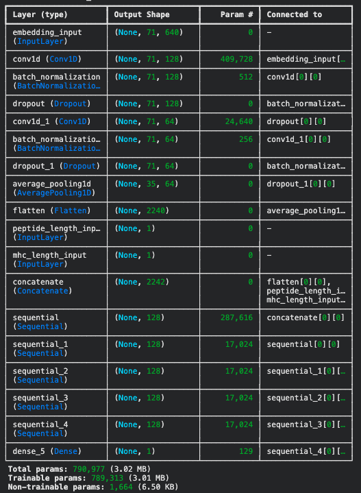
As we can see below, under the CNN architecture, the filter effectively compresses the embedding dimension from 640 down to 128, and then to 64. We set the padding to ‘same’ to retain the original sequence length of 71 after convolution. But if set to ‘valid’, the sequence length would reduce after each convolution layer, depending on the kernel size. The average pooling layer then reduces the sequence length dimension according to the pool size of 2 (basically halves it), and finally, we flatten the CNN output before concatenating it with the peptide and MHC2 lengths. This results in a feature vector of size 64 * 35 = 2240 from the CNN branch, which is then concatenated with the two length inputs, giving a total of 2242 features fed into the dense layers. Ultimately, the pooling layers help to prevent overfitting and save computational resources by reducing the dimensionality of the feature maps.
Compare this with the MLP-only model architecture that we will compare against:
# Define MLP layers
# Define a helper function for the repetitive dense -> batch norm -> dropout block
def make_dense_block(n_neurons, dropout_rate=0.2):
    return tf.keras.Sequential([
        tf.keras.layers.Dense(n_neurons, activation='relu', kernel_initializer='he_normal'),
        tf.keras.layers.BatchNormalization(),
        tf.keras.layers.Dropout(dropout_rate)
    ])

tf.random.set_seed(42)

dnn_model = tf.keras.Sequential([
    tf.keras.layers.Input(shape=X_train.shape[1:]),
    make_dense_block(512),
    make_dense_block(256),
    make_dense_block(128),
    make_dense_block(128),
    make_dense_block(128),
    tf.keras.layers.Dense(1)
])Set performance scheduling, early stopping, optimizer, compile model, and train the CNN + MLP model. The MLP-only model is trained with the same settings for comparison.
# Performance scheduling of learning rate
lr_scheduler = tf.keras.callbacks.ReduceLROnPlateau(factor=0.5, patience=5)

# Early stopping
early_stopping = tf.keras.callbacks.EarlyStopping(patience=10, restore_best_weights=True)

# Define optimizer
optimizer = tf.keras.optimizers.Adam(learning_rate=1e-4)

# Compile and train the model
cnn_model.compile(loss='mse', optimizer=optimizer, metrics=['RootMeanSquaredError', 'R2Score'])
fit_history = cnn_model.fit(train_tfds, epochs=100, validation_data=valid_tfds,
                            callbacks=[lr_scheduler, early_stopping])
Training CNN models is quite memory intensive. This specific data and model architecture required around 30-40 GB of GPU memory and 80-90 GB of system memory. With sufficient resources, the training completed in about 20 minutes per run on an NVIDIA A100 GPU.
Plot training metrics:
# Plot train and validation loss and RMSE across epochs
import matplotlib.pyplot as plt

fig, ax = plt.subplots(nrows=2, ncols=2, figsize=(8, 8))

pd.DataFrame(fit_history.history)[['loss', 'val_loss']].plot(
    grid=True, xlabel="Epoch", ax=ax[0, 0],
    style=["r--", "b-"])

pd.DataFrame(fit_history.history)[['RootMeanSquaredError', 'val_RootMeanSquaredError']].plot(
    grid=True, xlabel="Epoch", ax=ax[0, 1],
    style=["r--", "b-"])

pd.DataFrame(fit_history.history)[['R2Score', 'val_R2Score']].plot(
    grid=True, xlabel="Epoch", ax=ax[1, 0],
    style=["r--", "b-"])

pd.DataFrame(fit_history.history)[['learning_rate']].plot(
    grid=True, xlabel="Epoch", ax=ax[1, 1],
    style=["g-"])

ax[0, 0].set_ylabel('Loss')
ax[0, 0].set_title('Loss Over Epochs')
ax[0, 0].legend(['Training Loss', 'Validation Loss'])

ax[0, 1].set_ylabel('RMSE')
ax[0, 1].set_title('RMSE Over Epochs')
ax[0, 1].legend(['Training RMSE', 'Validation RMSE'])

ax[1, 0].set_ylabel('R2')
ax[1, 0].set_title('R2 Over Epochs')
ax[1, 0].legend(['Training R2', 'Validation R2'])

ax[1, 1].set_ylabel('Learning Rate')
ax[1, 1].set_title('Learning Rate Over Epochs')

plt.tight_layout()
plt.show().png)
The CNN + MLP model trained for the full 100 epochs, while the MLP-only model stopped early at epoch 80. Both models showed good convergence without overfitting.
Evaluate the model on the test set:
cnn_model.evaluate(X_test_inputs, y_test)Test Results:
- R2Score: 0.6219
- RootMeanSquaredError: 0.1606
- loss: 0.0258
For comparison, the MLP-only model achieved the following test results:
- R2Score: 0.5452
- RootMeanSquaredError: 0.1775
- loss: 0.0315
This indicates that, in this specific setting, incorporating CNN layers improved the model’s performance in predicting protein binding affinity.
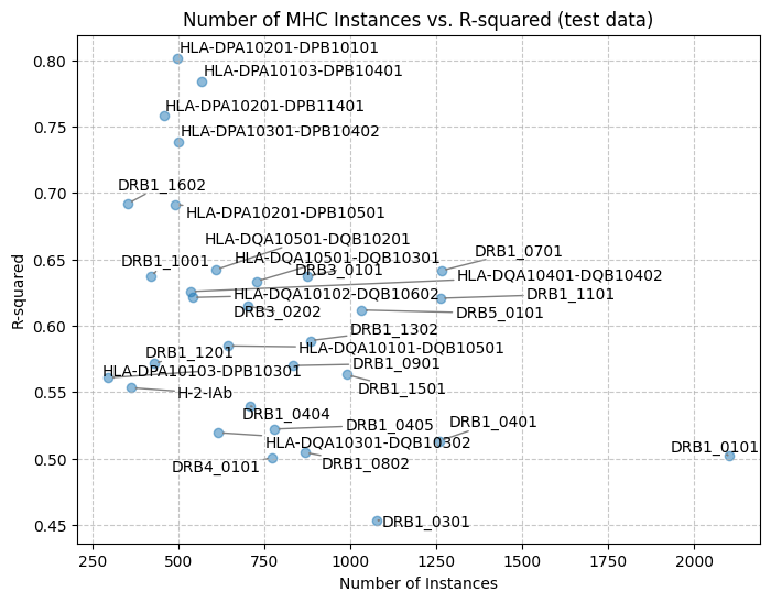
Let’s plot a comparison of MLP-only vs CNN + MLP prediction accuracy on the test set, stratified by MHC2 alleles. Higher R2Score indicates better prediction performance.
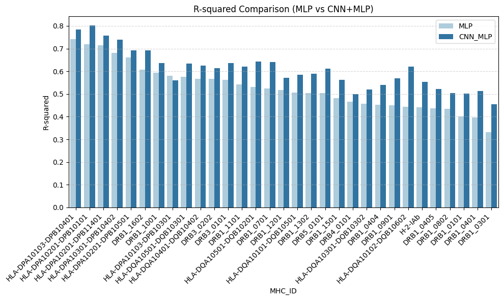
From the comparison plot, we can see that the CNN + MLP model generally provides better predictions across various MHC2 alleles compared to the MLP-only model.
Let’s look at one allele example on how well the CNN + MLP model predicts the affinity of HLA-DPA10201-DPB10101:
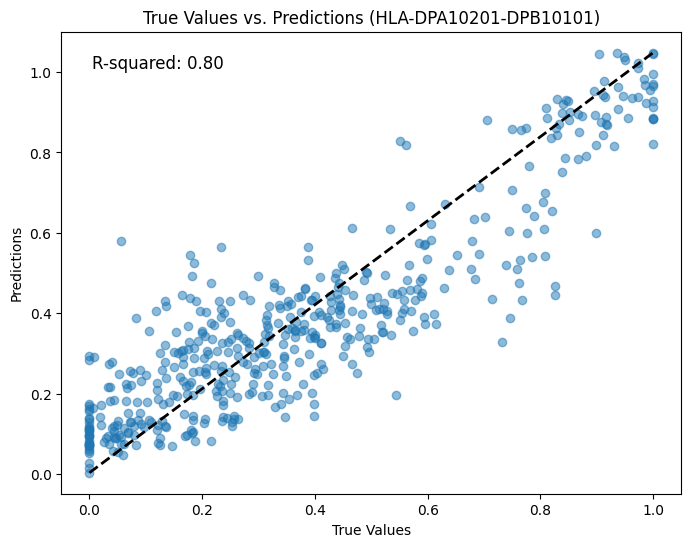
As we can see, the \(R^2\) = 0.8, which is an improvement over the MLP-only model of 0.72.
It is interesting to note that the MHC allele sample number does not correlate with the prediction performance, indicating that the model has learned meaningful patterns rather than just memorizing frequent alleles.
To compute the saliency maps, we will calculate the gradients of the model output with respect to the input embeddings. This will help us identify which amino acid positions in the peptide and MHC2 sequences are most influential for the binding affinity predictions.
We will first randomly select 5 high-affinity samples from the test set for saliency analysis:
# Select 5 samples from the test data where Y > 0.9
high_affinity_data = all_dat['test'][all_dat['test']['Y'] > 0.9].sample(5, random_state=42)

# Get the indices of these samples
sample_indices = high_affinity_data.index.values

print(f"Selected {len(high_affinity_data)} samples with Y > 0.9 for saliency analysis.")
print(high_affinity_data[['Peptide', 'MHC_ID', 'MHC', 'Y']])
Output:
Selected 5 samples with Y > 0.9 for saliency analysis.
               Peptide                 MHC_ID  \
21199  EKKYYAATQFEPLAA  HLA-DPA10301-DPB10402
5997   AFLIGANYLGKPKEQ              DRB1_0101
22257  DKRLAAYLMLMRSPS              DRB1_1501
8396   SQVNPITLTAALLLL              DRB1_0701
17575  NDKFTVFEGAFNKAI              DRB5_0101

                                      MHC         Y
21199  YMFFMFSGGAISNTLFGQFEYFDIEKVRMHLGMT  0.915458
5997   QEFFIASGAAVDAIMWLFLECYDLQRATYHVGFT  1.000000
22257  QEFFIASGAAVDAIMWPRFDYFDIQAATYHVVFT  1.000000
8396   QEFFIASGAAVDAIMWGYFELYVIDRQTVHVGFT  0.956843
17575  QEFFIASGAAVDAIMQDYFHDYDFDRATYHVGFT  1.000000
Now, we will extract the embeddings for these high-affinity samples:
# Get embeddings for these high affinity data
high_affinity_peptide = high_affinity_data['Peptide'].tolist()
high_affinity_mhc = high_affinity_data['MHC'].tolist()

max_len_pt = 37
max_len_mhc = 34

peptide_embeddings = extract_full_embedding(high_affinity_peptide, tokenizer, model, batch_size=1280, max_len=max_len_pt)
mhc_embeddings = extract_full_embedding(high_affinity_mhc, tokenizer, model, batch_size=1280, max_len=max_len_mhc)

# Concatenate the embeddings
X_high_affinity_embeddings = np.concatenate([peptide_embeddings, mhc_embeddings], axis=1)

# Extract corresponding sequence lengths
X_high_affinity_pt_len = high_affinity_data['Peptide'].apply(len).values
X_high_affinity_mhc_len = high_affinity_data['MHC'].apply(len).values
Define a helper function to compute saliency maps:
import tensorflow as tf
import numpy as np
import matplotlib.pyplot as plt
import seaborn as sns

def calculate_saliency_map(model: tf.keras.Model,
                           embedding_data: np.ndarray,
                           peptide_len_data: np.ndarray,
                           mhc_len_data: np.ndarray,
                           target_idx: int = 0) -> np.ndarray:

    """Calculates saliency map for a given input using the trained model."""

    # Convert numpy arrays to TensorFlow tensors and ensure float32
    input_embeddings_tensor = tf.convert_to_tensor(embedding_data, dtype=tf.float32)
    peptide_len_tensor = tf.convert_to_tensor(peptide_len_data, dtype=tf.float32)
    mhc_len_tensor = tf.convert_to_tensor(mhc_len_data, dtype=tf.float32)

    with tf.GradientTape() as tape:
        tape.watch(input_embeddings_tensor) # Watch only the embeddings for saliency

        # Pass all inputs to the model for prediction of Y
        predictions = model((input_embeddings_tensor, peptide_len_tensor, mhc_len_tensor))

        # Select the target output if there are multiple outputs or a specific class
        target_output = predictions[:, target_idx]

    # Calculate gradients of the target output with respect to the input embeddings
    gradients = tape.gradient(target_output, input_embeddings_tensor)

    # Take the mean across the embedding dimension to get a single saliency score per amino acid position
    saliency = tf.reduce_mean(gradients, axis=-1) # Take mean along last axis: embedding_dim

return saliency.numpy().flatten()# Package inputs for the model's predict method
X_high_affinity_inputs = (X_high_affinity_embeddings, X_high_affinity_pt_len, X_high_affinity_mhc_len)
# Predictions for selected samples
y_pred_high_affinity = cnn_model.predict(X_high_affinity_inputs)Compute and plot the saliency maps for each selected high-affinity sample:
fig, axes = plt.subplots(nrows=len(high_affinity_data), ncols=2, figsize=(18, len(high_affinity_data) * 3))
fig.suptitle('Saliency Maps for High Affinity Peptide-MHC Pairs (Y > 0.9)', fontsize=16)

# Ensure axes is always 2D even for a single row
if len(high_affinity_data) == 1:
    axes = np.array([axes])

for i in range(len(high_affinity_data)):
    sample_info = high_affinity_data.iloc[i]
    peptide_sequence = sample_info['Peptide']
    mhc_sequence = sample_info['MHC']
    mhc_id = sample_info['MHC_ID']
    y_true_sample = sample_info['Y']
    y_pred_sample = y_pred_high_affinity[i][0] # Access pre-calculated prediction

    # Get one sample's embeddings and lengths at a time
    current_embedding_data = X_high_affinity_embeddings[i:i+1]
    current_peptide_len_data = X_high_affinity_pt_len[i:i+1]
    current_mhc_len_data = X_high_affinity_mhc_len[i:i+1]

    # Calculate saliency map using the updated function signature
    # Normalize with a constant to enhance visualization
    beta = 1e5
    saliency_scores = calculate_saliency_map(cnn_model,
                                             current_embedding_data,
                                             current_peptide_len_data,
                                             current_mhc_len_data) * beta

    peptide_len = len(peptide_sequence)
    mhc_len = len(mhc_sequence)

    # Correctly slice saliency scores based on actual sequence lengths
    peptide_saliency = saliency_scores[:peptide_len]
    mhc_saliency = saliency_scores[max_len_pt : max_len_pt + mhc_len]

    annot_settings = {"rotation": 90}

    # Plot for Peptide Saliency
    sns.heatmap(
        [peptide_saliency],
        cmap='coolwarm',
        annot=True,
        annot_kws=annot_settings,
        fmt=".2f",
        xticklabels=list(peptide_sequence),
        yticklabels=['Peptide'],
        cbar_kws={'label': 'Saliency Score'},
        ax=axes[i, 0]
    )
    axes[i, 0].set_title(f'Sample {i+1} - Peptide: {peptide_sequence}\nTrue Y: {y_true_sample:.2f}, Pred Y: {y_pred_sample:.2f}')
    axes[i, 0].tick_params(axis='x', rotation=0)

    # Plot for MHC Saliency
    sns.heatmap(
        [mhc_saliency],
        cmap='coolwarm',
        annot=True,
        annot_kws=annot_settings,
        fmt=".2f",
        xticklabels=list(mhc_sequence),
        yticklabels=['MHC'],
        cbar_kws={'label': 'Saliency Score'},
        ax=axes[i, 1]
    )
    axes[i, 1].set_title(f'Sample {i+1} - MHC: {mhc_sequence}\nMHC ID: {mhc_id}')
    axes[i, 1].tick_params(axis='x', rotation=0)

plt.tight_layout(rect=[0, 0.03, 1, 0.95]) # Adjust layout to make space for suptitle
plt.show()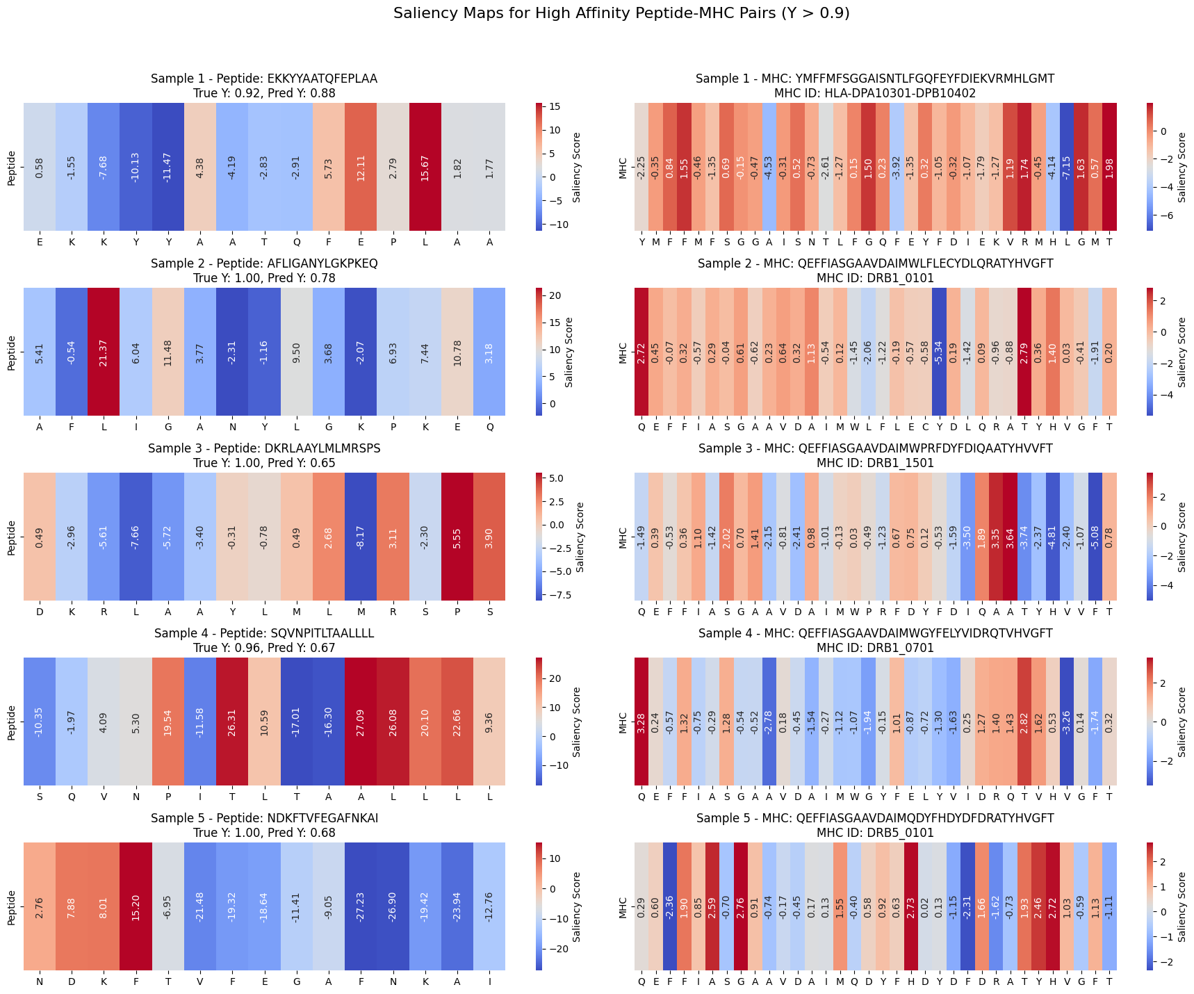
Positive saliency scores (red) indicate that the amino acids are positively correlated with a higher binding affinity, while negative scores (blue) suggest that those amino acids contribute to lower binding affinity.
Next, let’s perform In Silico Mutagenesis (ISM) analysis to see how single amino acid mutations affect the predicted binding affinity. Instead of mutating every position, which will be computationally expensive, we will focus on mutating only the most salient positions (highest saliency score) in the peptide sequences for each sample.
First, generate a dictionary of the most disruptive mutations for each amino acid:
# A dictionary that suggests the most disruptive mutagenesis for each a.a.
disruptive_mutations = {
    'A': 'W', # Small nonpolar -> Bulkiest nonpolar/aromatic
    'R': 'D', # Positively charged -> Negatively charged
    'N': 'F', # Polar uncharged -> Hydrophobic aromatic
    'D': 'R', # Negatively charged -> Positively charged
    'C': 'S', # Disulfide bond former -> Similar size but non-disulfide/polar
    'E': 'K', # Negatively charged -> Positively charged
    'Q': 'W', # Polar uncharged -> Bulkiest nonpolar/aromatic
    'G': 'P', # Flexible -> Conformational constraint
    'H': 'D', # Positively charged -> Negatively charged (pH depending)
    'I': 'E', # Hydrophobic -> Negatively charged hydrophilic
    'L': 'K', # Hydrophobic -> Positively charged hydrophilic
    'K': 'D', # Positively charged -> Negatively charged
    'M': 'E', # Nonpolar/sulfur -> Negatively charged hydrophilic
    'F': 'E', # Hydrophobic aromatic -> Negatively charged hydrophilic
    'P': 'G', # Conformational constraint -> Flexible
    'S': 'L', # Polar uncharged -> Hydrophobic
    'T': 'I', # Polar uncharged -> Hydrophobic
    'W': 'A', # Bulkiest nonpolar -> Smallest nonpolar
    'Y': 'D', # Aromatic/polar -> Negatively charged
    'V': 'E'  # Hydrophobic -> Negatively charged hydrophilic
}
Perform ISM on the top salient positions in the peptide sequences:
# Find aa with the highest saliency score across all samples
max_scores_aa_pos_pt = {}
for i in range(len(high_affinity_data)):
  sample_info = high_affinity_data.iloc[i]
  peptide_sequence = sample_info['Peptide']
  current_embedding_data = X_high_affinity_embeddings[i:i+1]
  current_peptide_len_data = X_high_affinity_pt_len[i:i+1]
  current_mhc_len_data = X_high_affinity_mhc_len[i:i+1]
  saliency = calculate_saliency_map(cnn_model, current_embedding_data, current_peptide_len_data, current_mhc_len_data)
  max_score_pos = saliency[:current_peptide_len_data[0]].argmax().tolist()
  max_score_aa = peptide_sequence[max_score_pos]
  max_scores_aa_pos_pt[sample_info['Peptide_ID'].tolist()] = {max_score_aa: max_score_pos}

print("Identified highest saliency amino acids and their positions:")
display(max_scores_aa_pos_pt)
Output:
Identified highest saliency amino acids and their positions:
{60550: {'L': 12},
 117646: {'L': 2},
 51178: {'P': 13},
 73939: {'A': 10},
26350: {'F': 3}}mutated_peptide_predictions = []
for i, (peptide_id, saliency_info) in enumerate(max_scores_aa_pos_pt.items()):
# Get original sample info
sample_row = high_affinity_data[high_affinity_data['Peptide_ID'] == peptide_id].iloc[0]
original_peptide = sample_row['Peptide']
original_mhc = sample_row['MHC']
original_y_pred = y_pred_high_affinity[high_affinity_data['Peptide_ID'] == peptide_id].flatten()[0]
# Get the AA with highest saliency and its position
saliency_aa = list(saliency_info.keys())[0]
saliency_pos = list(saliency_info.values())[0]
# Determine the disruptive mutation
disruptive_aa = disruptive_mutations.get(saliency_aa, 'A') # Default to Alanine if not in dict
# Create mutated peptide sequence
mutated_peptide_sequence_list = list(original_peptide)
mutated_peptide_sequence_list[saliency_pos] = disruptive_aa
mutated_peptide = ''.join(mutated_peptide_sequence_list)
# --- Extract embeddings for the mutated peptide ---
# Ensure original MHC embeddings are reused to isolate peptide effect
original_mhc_embeddings = extract_full_embedding([original_mhc], tokenizer, model, batch_size=1, max_len=max_len_mhc)
# Extract embeddings for the mutated peptide
mutated_peptide_embeddings = extract_full_embedding([mutated_peptide], tokenizer, model, batch_size=1, max_len=max_len_pt)
# Concatenate mutated peptide embeddings with original MHC embeddings
X_mutated_combined_embeddings = np.concatenate([mutated_peptide_embeddings, original_mhc_embeddings], axis=1)
# Get sequence lengths for mutated peptide and original MHC
mutated_peptide_len = np.array([len(mutated_peptide)])
original_mhc_len = np.array([len(original_mhc)])
# Package inputs for prediction
X_mutated_inputs = (
X_mutated_combined_embeddings,
tf.convert_to_tensor(mutated_peptide_len, dtype=tf.float32),
tf.convert_to_tensor(original_mhc_len, dtype=tf.float32)
)
# Predict binding affinity for the mutated peptide
mutated_y_pred = cnn_model.predict(X_mutated_inputs).flatten()[0]
mutated_peptide_predictions.append({
'Peptide_ID': peptide_id,
'Original_Peptide': original_peptide,
'Mutated_Peptide': mutated_peptide,
'Saliency_AA': saliency_aa,
'Saliency_Pos': saliency_pos + 1,
'Disruptive_AA': disruptive_aa,
'Original_Pred_Y': original_y_pred,
'Mutated_Pred_Y': mutated_y_pred,
'Change_in_Y': mutated_y_pred - original_y_pred
})
mutated_predictions_df = pd.DataFrame(mutated_peptide_predictions)
print(mutated_predictions_df)Output:
   Peptide_ID Original_Peptide  Mutated_Peptide Saliency_AA  Saliency_Pos  \
0       60550  EKKYYAATQFEPLAA  EKKYYAATQFEPKAA           L            13
1      117646  AFLIGANYLGKPKEQ  AFKIGANYLGKPKEQ           L             3
2       51178  DKRLAAYLMLMRSPS  DKRLAAYLMLMRSGS           P            14
3       73939  SQVNPITLTAALLLL  SQVNPITLTAWLLLL           A            11
4       26350  NDKFTVFEGAFNKAI  NDKETVFEGAFNKAI           F             4

  Disruptive_AA  Original_Pred_Y  Mutated_Pred_Y  Change_in_Y
0             K         0.879057        0.721061    -0.157996
1             K         0.782684        0.729118    -0.053567
2             G         0.652823        0.643233    -0.009590
3             W         0.665965        0.581599    -0.084366
4             E         0.678189        0.355576    -0.322613
Plot the changes in predicted binding affinity due to the mutations:
import matplotlib.pyplot as plt
import seaborn as sns
from adjustText import adjust_text

plt.figure(figsize=(8, 6))
sns.scatterplot(
    data=mutated_predictions_df,
    x='Original_Pred_Y',
    y='Mutated_Pred_Y',
    hue='Change_in_Y',
    s=200,
    palette='coolwarm',
    legend='full'
)

# Add a diagonal line for reference (where Y_original == Y_mutated)
plt.plot([0, 1], [0, 1], 'k--', lw=2, alpha=0.5, label='No Change')

# Annotate points with Peptide_ID or a combination of info
texts = []
for idx, row in mutated_predictions_df.iterrows():
    label = f"{row['Original_Peptide']}\n{row['Saliency_AA']}{row['Saliency_Pos']}->{row['Disruptive_AA']}"
    texts.append(plt.text(row['Original_Pred_Y'], row['Mutated_Pred_Y'], label, fontsize=10))

adjust_text(texts, arrowprops=dict(arrowstyle="-", color='gray', lw=1))

plt.title('Predicted Binding Affinity: Original vs. Mutated Peptides')
plt.xlabel('Original Predicted Y')
plt.ylabel('Mutated Predicted Y')
plt.grid(True, linestyle='--', alpha=0.6)
plt.xlim(0.3, 1)
plt.ylim(0.3, 1)
plt.axhline(y=0.5, color='gray', linestyle=':', lw=1, alpha=0.7)
plt.axvline(x=0.5, color='gray', linestyle=':', lw=1, alpha=0.7)
plt.legend(title='Change in Y')
plt.show()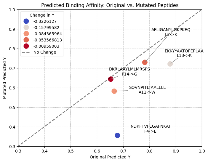
As we can see from the ISM analysis, mutating the most salient amino acid positions in the peptide sequences generally leads to a decrease in predicted binding affinity, as indicated by the points falling below the diagonal line. Some mutations result in significant drops in predicted affinity, while others are less impactful. However, we are only mutating a single position here, and multiple mutations may have a more pronounced effect. This analysis provides a hypothesis for experimental validation of key residues involved in peptide-MHC binding.
Incorporating convolutional neural networks (CNNs) into the protein binding prediction model improved performance compared to a MLP-only approach. By retaining the 2D structure of the ESM2 embeddings and applying 1D convolutional layers, the model was able to capture local sequence patterns that are important for binding affinity prediction. The CNN + MLP model achieved higher R2 scores and lower RMSE on the test set, demonstrating its effectiveness.
It is important to note that further hyperparameter tuning for either model could yield different results. Additionally, exploring other architectures, such as attention mechanisms, could provide additional insights into modeling protein binding affinity.