library(tidyverse)
library(data.table)
library(ggpubr)
library(caret)
library(doParallel)

# Load data from the files directory
load("files/CCLE_24Q2_GE_match_sample_info.RData")
load("files/PRISM_24Q2_compound_screen_match_sample_info.RData")
cmpd_dat <- read_csv("files/Repurposing_Public_24Q2_Extended_Primary_Compound_List.csv")
load("files/sample_info_match_biomarkers.RData")Machine learning for drug sensitivity prediction (Part 3): Training an Elastic Net gene expression model to predict Erlotinib sensitivity
R
DepMap
Machine Learning
Elastic Net
Caret
In my previous posts (part 1 and part 2), I explored whether using autoencoders (AE) to compress high-dimensional multi-omics data could improve the performance of drug sensitivity prediction models. In my specific context, I showed that using AE did not necessarily improve model performance compared to using a common feature selection method.
In this post, I will use the best-performing model from my previous analyses (elastic net using features selected by Pearson correlation), and apply it to all available DepMap data to generate predictions for cell lines without measured drug sensitivity. I will then see if these predictions provide additional useful insights beyond the measured data.
I will demonstrate how to use R’s Caret package to train an elastic net model with hyperparameter tuning via cross-validation.
Aim 1: Apply the elastic net model to all available DepMap data to generate Erlotinib sensitivity predictions
Data location (pre-processed for this post): https://zenodo.org/records/17970100
Load data and libraries
Preprocessing
First, we remove low variance genes and any cell lines containing NAs.
# Remove low variance genes
ge_var <- apply(ccle_ge_match_sam, 2, var, na.rm = TRUE) # calculate variance for each gene
ge_dat_hv <- ccle_ge_match_sam[, which(ge_var > quantile(ge_var, 0.2))] # select high variance genes

# Remove any cell lines (rows) that contains NAs
ge_dat_hv <- ge_dat_hv |>
    na.omit() |>
    as.data.frame()

# Match data
match_idx <- match(rownames(ge_dat_hv), sample_info$StrippedCellLineName)
sample_info_filt <- sample_info[match_idx, ]
prism_dat_match_sam_filt <- prism_dat_match_sam[match_idx, ]

# Verify alignment
all(rownames(ge_dat_hv) == sample_info_filt$StrippedCellLineName)
[1] TRUENow we prepare the drug response data for Erlotinib.
cmpd_id <- cmpd_dat |>
    filter(Drug.Name == "ERLOTINIB") |>
    pull(IDs)
drug_LFC <- prism_dat_match_sam_filt |> pull(cmpd_id) # Erlotinib LFC

# Remove NAs in drug response
valid_idx <- which(!is.na(drug_LFC))
ge_dat_final <- ge_dat_hv[valid_idx, ]
drug_LFC_final <- drug_LFC[valid_idx]
sample_info_final <- sample_info_filt[valid_idx, ]

# Verify alignment
all(rownames(ge_dat_final) == sample_info_final$StrippedCellLineName)
[1] TRUE# Check drug response distribution
ggplot(data.frame(Erlotinib_LFC = drug_LFC_final), aes(x = Erlotinib_LFC)) +
geom_density(fill = "purple", alpha = 0.7) +
theme_classic(base_size = 20) +
labs(title = "Density of Erlotinib LFC", x = "Erlotinib LFC", y = "Density")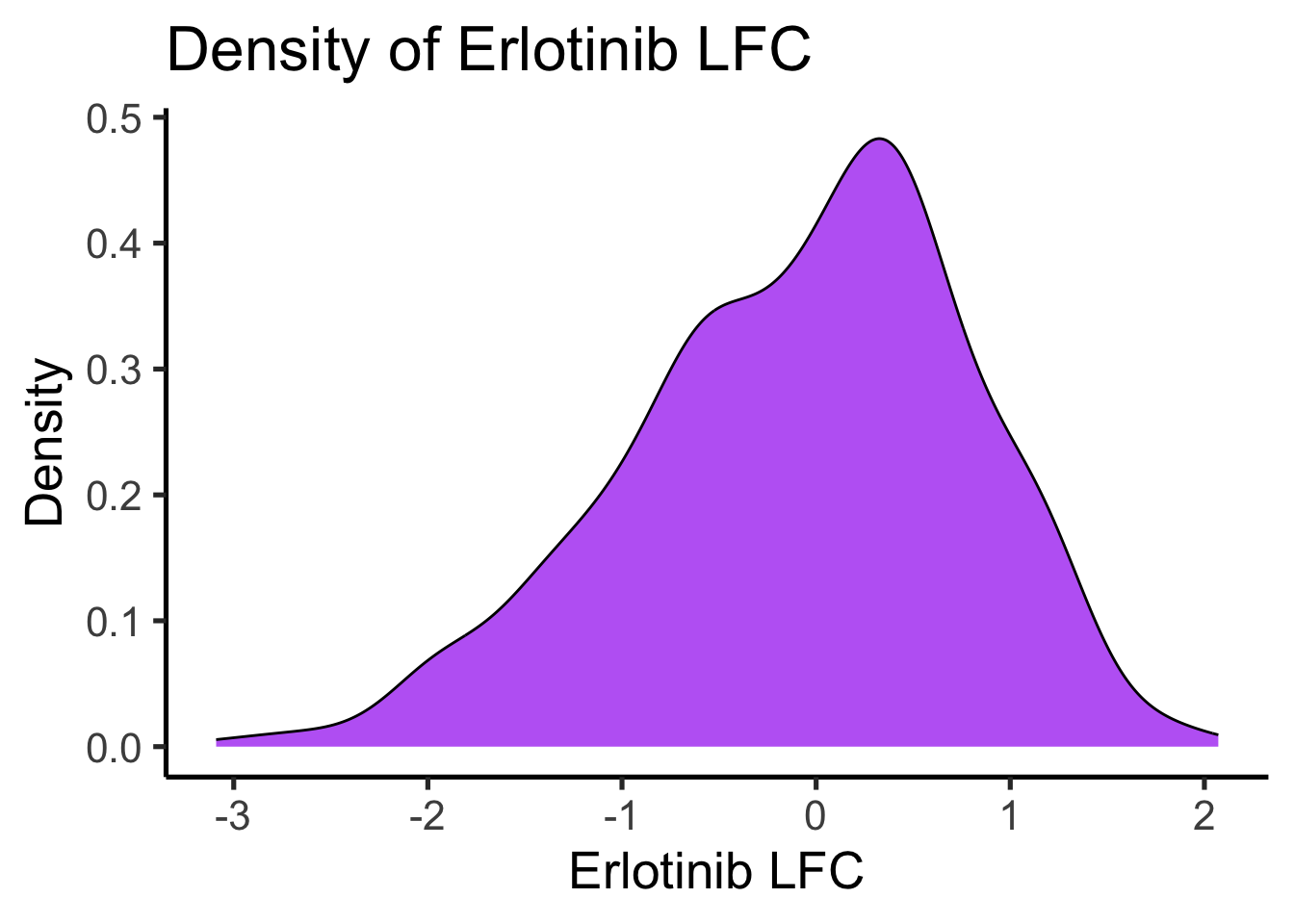
Feature Selection
We select the top predictors correlating with the drug response.
# Select top predictors correlating with drug response, Pearson correlation > 0.1
cor_values <- apply(ge_dat_final, 2, function(x) cor(x, drug_LFC_final, method = "pearson"))
cor_values <- abs(cor_values)
ggplot(data.frame(Correlation = cor_values), aes(x = Correlation)) +
    geom_density(fill = "darkgreen", alpha = 0.7) +
    theme_classic(base_size = 20) +
    labs(title = "Density of Gene-Drug Correlation Values", x = "Absolute Pearson Correlation", y = "Density")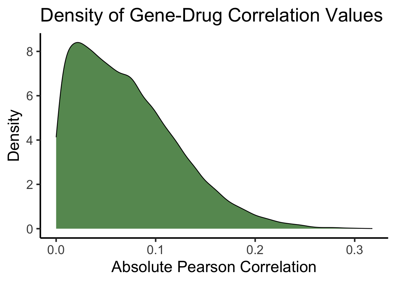
top_predictors <- names(cor_values)[which(cor_values > 0.1)]
ge_dat_final <- ge_dat_final |> select(all_of(top_predictors))
Elastic Net Hyperparameter Tuning
We perform hyperparameter tuning using caret.
Note: The training step is computationally intensive and is not evaluated here. We load the pre-trained model for subsequent analysis.
# Elastic net hyperparameter tuning with caret
detectCores()
cl <- makePSOCKcluster(22)
registerDoParallel(cl)

glmnetGrid <- expand.grid(
    .lambda = round(seq(0.005, 5, length = 30), 3),
    .alpha = round(seq(0, 0.1, length = 10), 3)
)

set.seed(524)
enet_full_model <- train(ge_dat_final, drug_LFC_final,
    method = "glmnet",
    tuneGrid = glmnetGrid,
    preProcess = c("center", "scale"),
    metric = "Rsquared",
    trControl = trainControl(method = "repeatedcv", number = 10, repeats = 10)
)
stopCluster(cl)

# Save the final model (Already saved in files/)
# save(enet_full_model, file = "files/enet_full_model_erlotinib.RData")
Model Analysis
Let’s examine the tuning results and the best hyperparameters.
# Load the pre-trained model
load("files/enet_full_model_erlotinib.RData")

# View hyperparameter tuning results
enet_full_model$results |> arrange(desc(Rsquared)) |> head(20) |> gt::gt()| alpha | lambda | RMSE | Rsquared | MAE | RMSESD | RsquaredSD | MAESD |
|---|---|---|---|---|---|---|---|
| 0.011 | 1.038 | 0.7246115 | 0.3234841 | 0.5678419 | 0.06244775 | 0.09552666 | 0.05504541 |
| 0.011 | 1.211 | 0.7243195 | 0.3231371 | 0.5668798 | 0.06237722 | 0.09620741 | 0.05451755 |
| 0.011 | 0.866 | 0.7259216 | 0.3227335 | 0.5697183 | 0.06251476 | 0.09492452 | 0.05557950 |
| 0.011 | 1.383 | 0.7246391 | 0.3221409 | 0.5665405 | 0.06232075 | 0.09689575 | 0.05382773 |
| 0.011 | 1.555 | 0.7254462 | 0.3205662 | 0.5668465 | 0.06223333 | 0.09753524 | 0.05317660 |
| 0.011 | 0.694 | 0.7287441 | 0.3204541 | 0.5731421 | 0.06255456 | 0.09446370 | 0.05612583 |
| 0.011 | 1.727 | 0.7265929 | 0.3185779 | 0.5676531 | 0.06210627 | 0.09802932 | 0.05253257 |
| 0.022 | 0.694 | 0.7276708 | 0.3185370 | 0.5695071 | 0.06120405 | 0.09481046 | 0.05397744 |
| 0.022 | 0.522 | 0.7298551 | 0.3180041 | 0.5726883 | 0.06144171 | 0.09315651 | 0.05466701 |
| 0.022 | 0.866 | 0.7277250 | 0.3168255 | 0.5686165 | 0.06109334 | 0.09620112 | 0.05314454 |
| 0.011 | 1.900 | 0.7279475 | 0.3163917 | 0.5686306 | 0.06199278 | 0.09836348 | 0.05195792 |
| 0.011 | 0.522 | 0.7339054 | 0.3158314 | 0.5786809 | 0.06262747 | 0.09381218 | 0.05677975 |
| 0.033 | 0.522 | 0.7303634 | 0.3142904 | 0.5715719 | 0.06047743 | 0.09405803 | 0.05348058 |
| 0.011 | 2.072 | 0.7294330 | 0.3141275 | 0.5697778 | 0.06194162 | 0.09867437 | 0.05146113 |
| 0.022 | 1.038 | 0.7289549 | 0.3140533 | 0.5692525 | 0.06118321 | 0.09735362 | 0.05229037 |
| 0.022 | 0.349 | 0.7362917 | 0.3135250 | 0.5805138 | 0.06171108 | 0.09216744 | 0.05541844 |
| 0.033 | 0.694 | 0.7296913 | 0.3129244 | 0.5700855 | 0.06080031 | 0.09625073 | 0.05273691 |
| 0.011 | 2.244 | 0.7309768 | 0.3118847 | 0.5711072 | 0.06195602 | 0.09901043 | 0.05102660 |
| 0.044 | 0.522 | 0.7306761 | 0.3116728 | 0.5711300 | 0.06048624 | 0.09528180 | 0.05289960 |
| 0.033 | 0.349 | 0.7355536 | 0.3116308 | 0.5781206 | 0.06063449 | 0.09156073 | 0.05410146 |
The best hyperparameters for the model were alpha = 0.011 and lambda = 1.038. This indicates that the model prefers a nearly ridge regression approach (alpha close to 0) with moderate regularization (lambda value). This makes sense given that the predictors were pre-selected based on correlation with the response, so we want to retain most predictors while controlling for multicollinearity.
# Plot tuning results
ggplot(enet_full_model) +
    theme_classic(base_size = 20) +
    labs(title = "Elastic Net tuning")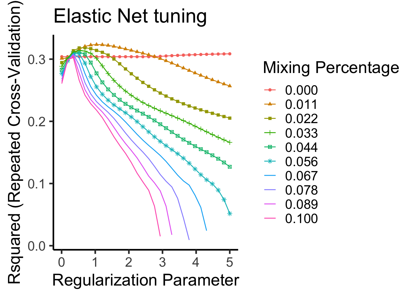
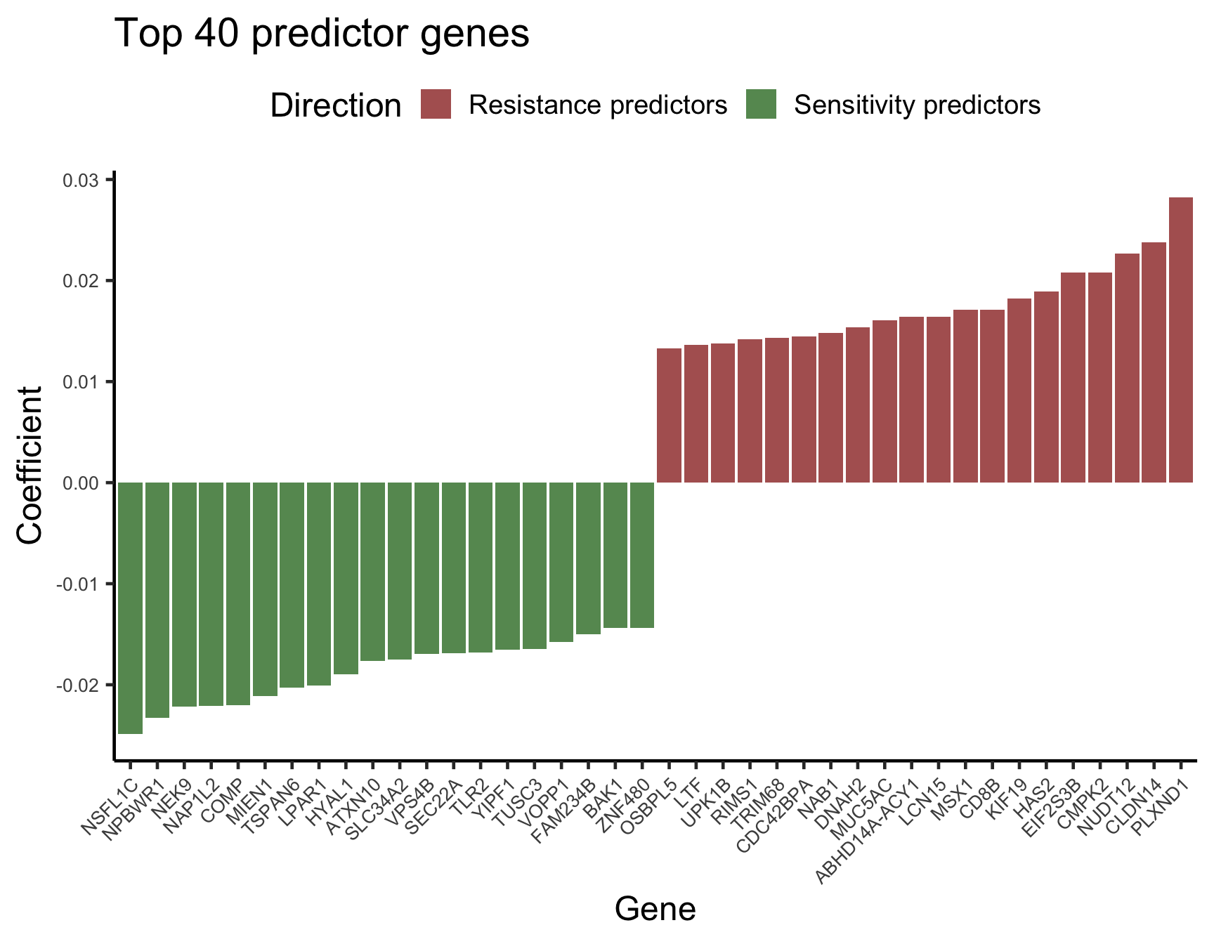
A major advantage of a linear model like elastic net is its interpretability. The coefficients correspond to how important each gene is for predicting Erlotinib sensitivity.
final_coef <- as.matrix(coef(enet_full_model$finalModel, s = enet_full_model$bestTune$lambda))[-1, ]
final_coef_df <- data.frame(
    Gene = names(final_coef),
    Coefficient = final_coef
)

# Plot a bar plot for the top 20 sensitivity and top 20 resistance predictor genes
final_coef_sorted <- final_coef[order(final_coef, decreasing = TRUE)]
top20_pos_coef <- head(final_coef_sorted[final_coef_sorted > 0], 20)
top20_neg_coef <- tail(final_coef_sorted[final_coef_sorted < 0], 20)

top_coef_df <- data.frame(
    Gene = c(names(top20_pos_coef), names(top20_neg_coef)),
    Coefficient = c(top20_pos_coef, top20_neg_coef),
    Direction = c(rep("Resistance predictors", length(top20_pos_coef)), rep("Sensitivity predictors", length(top20_neg_coef)))
)

ggplot(top_coef_df, aes(x = reorder(Gene, Coefficient), y = Coefficient, fill = Direction)) +
    geom_bar(stat = "identity", alpha = 0.7) +
    theme_classic(base_size = 18) +
    labs(
        title = "Top 40 predictor genes",
        x = "Gene",
        y = "Coefficient"
    ) +
    scale_fill_manual(values = c("Sensitivity predictors" = "darkgreen", "Resistance predictors" = "darkred")) +
    theme(
        legend.position = "top",
        axis.text.x = element_text(angle = 45, hjust = 1),
        axis.text = element_text(size = 10)
    )
Prediction on All Cell Lines
We now use the trained model to predict Erlotinib sensitivity for all CCLE cell lines with available RNA expression data.
# Predict on all CCLE cell lines with available RNA expression
all_ccle_ge <- ccle_ge_match_sam |> as.data.frame()
all_ccle_ge <- all_ccle_ge |>
    select(all_of(top_predictors)) |>
    na.omit() # 1517 cell lines with complete GE data

enet_pred_all_ccle <- predict(enet_full_model, newdata = all_ccle_ge)

# Save predicted Erlotinib LFC for all CCLE cell lines
predicted_erlotinib_df <- data.frame(
    Cell_Line = rownames(all_ccle_ge),
    Predicted_Erlotinib_LFC = enet_pred_all_ccle
)
# fwrite(predicted_erlotinib_df, "files/predicted_erlotinib_LFC_all_CCLE_cell_lines.csv", sep = ",", row.names = FALSE, quote = FALSE)
Aim 2: Evaluate whether the predicted Erlotinib sensitivity provides additional insights beyond the measured data
Comparison of Actual vs. Predicted
# Load actual and predicted Erlotinib LFC data
actual_erlotinib_df <- data.frame(
    Cell_Line = rownames(ge_dat_final),
    Actual_Erlotinib_LFC = drug_LFC_final
)

# If we didn't run the prediction above, we could load it:
# predicted_erlotinib_df <- fread("files/predicted_erlotinib_LFC_all_CCLE_cell_lines.csv", data.table = FALSE)

# Merge actual and predicted data
erlotinib_compare_df <- merge(actual_erlotinib_df, predicted_erlotinib_df, by = "Cell_Line", all = TRUE)

# Add cancer lineage information
erlotinib_compare_df <- erlotinib_compare_df |> left_join(sample_info |> select(StrippedCellLineName, OncotreeLineage),
    by = c("Cell_Line" = "StrippedCellLineName")
)

# Add EGFR mutation status
# Note: Using tryCatch or existence check in case file is missing in user environment
if (file.exists("files/CCLE_24Q2_HOTMUT_match_sample_info.RData")) {
    load("files/CCLE_24Q2_HOTMUT_match_sample_info.RData")
    egfr_mutation_status <- hotmut_dat_match_sam |>
        rownames_to_column(var = "Cell_Line") |>
        select(Cell_Line, EGFR) |>
        mutate(EGFR_Mutation_Status = recode(as.factor(EGFR), `0` = "Wildtype", `1` = "Heterozygous Mutant", `2` = "Homozygous Mutant")) |>
        select(Cell_Line, EGFR_Mutation_Status)
    erlotinib_compare_df <- erlotinib_compare_df |> left_join(egfr_mutation_status, by = "Cell_Line")
} else {
    warning("files/CCLE_24Q2_HOTMUT_match_sample_info.RData not found. Skipping EGFR analysis.")
}

# Plot actual vs predicted Erlotinib LFC for cell lines with actual data
plot_df <- erlotinib_compare_df |> filter(!is.na(Actual_Erlotinib_LFC))
ggplot(plot_df, aes(x = Actual_Erlotinib_LFC, y = Predicted_Erlotinib_LFC)) +
    geom_point(color = "steelblue", size = 3, alpha = 0.7) +
    theme_classic(base_size = 20) +
    theme(plot.title = element_text(size = 20)) +
    labs(
        title = "Elastic Net prediction of Erlotinib LFC",
        x = "Actual Erlotinib LFC",
        y = "Predicted Erlotinib LFC"
    ) +
    stat_cor(method = "pearson", label.x.npc = "left", label.y.npc = "top", size = 6, color = "darkred") +
    geom_smooth(method = "lm", color = "darkred", se = TRUE)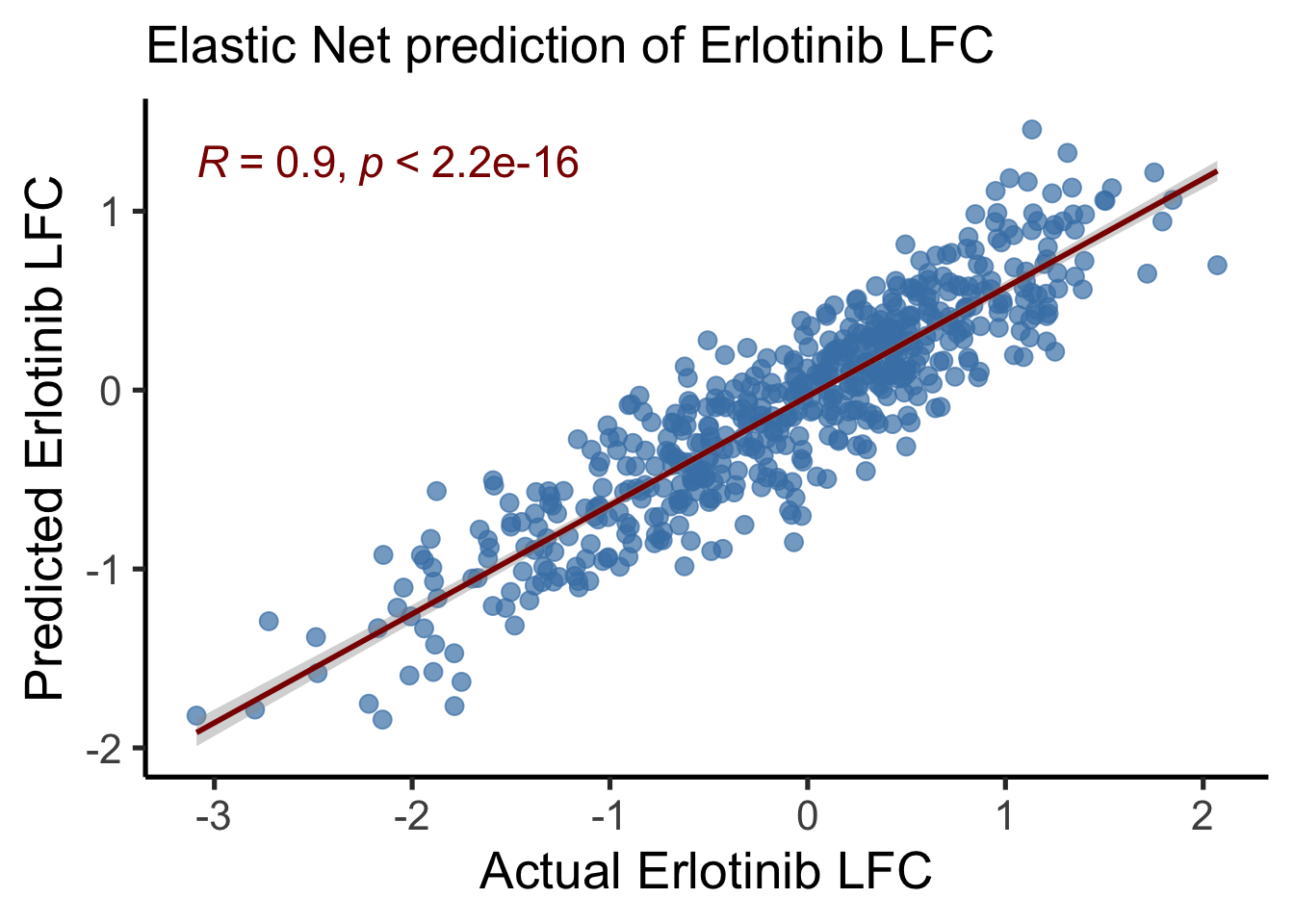
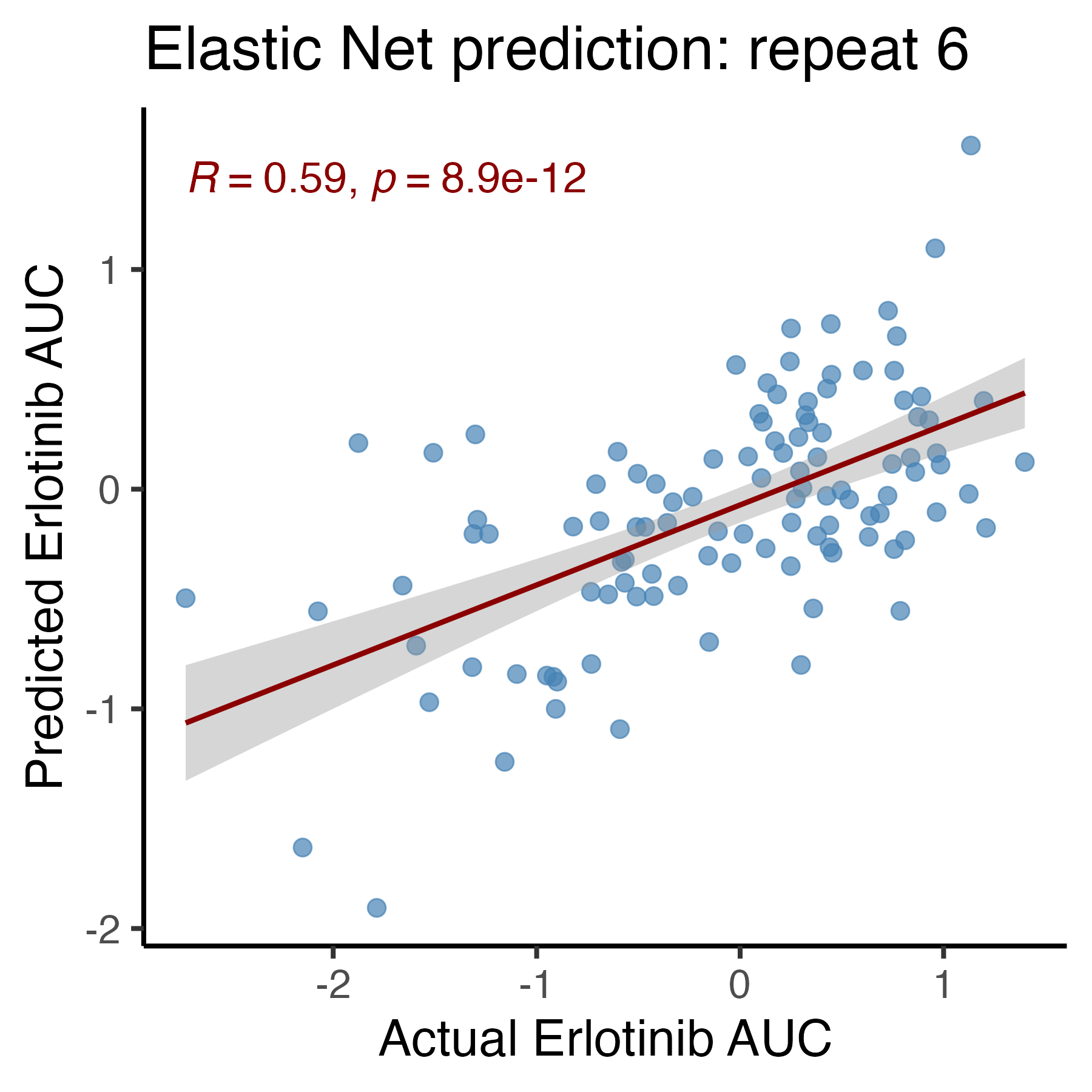
Note: This prediction performance result is evaluated on the training data, so it is expected to be better than on independent test data (overfitting). It is important to always evaluate model performance on independent test data. From my previous post, the prediction performance on independent test data looks like this (not bad but not as good as training data):
Cancer Lineage Distribution
We compare the cancer lineages covered by the actual measured data versus the predicted data.
actual_lineages <- erlotinib_compare_df |>
    filter(!is.na(Actual_Erlotinib_LFC)) |>
    select(Cell_Line, OncotreeLineage) |>
    distinct()
predicted_lineages <- erlotinib_compare_df |>
    select(Cell_Line, OncotreeLineage) |>
    distinct()

actual_lineage_counts <- actual_lineages |>
    group_by(OncotreeLineage) |>
    summarise(Count = n()) |>
    mutate(Type = "Actual data")
predicted_lineage_counts <- predicted_lineages |>
    group_by(OncotreeLineage) |>
    summarise(Count = n()) |>
    mutate(Type = "Predicted data")
lineage_counts_df <- rbind(actual_lineage_counts, predicted_lineage_counts) |> filter(OncotreeLineage != "")

# Make missing lineage in actual data have count 0
all_lineages <- unique(lineage_counts_df$OncotreeLineage)
for (lineage in all_lineages) {
    if (!(lineage %in% actual_lineage_counts$OncotreeLineage)) {
        lineage_counts_df <- rbind(lineage_counts_df, data.frame(OncotreeLineage = lineage, Count = 0, Type = "Actual data"))
    }
}

ggplot(lineage_counts_df, aes(x = reorder(OncotreeLineage, -Count), y = Count, fill = Type)) +
    geom_bar(stat = "identity", position = position_dodge()) +
    theme_classic(base_size = 18) +
    labs(
        title = "Cancer Lineage Distribution",
        x = "Cancer Lineage",
        y = "Number of Cell Lines"
    ) +
    geom_text(aes(label = Count, color = Type), position = position_dodge(width = 0.9), vjust = -0.5, size = 3) +
    scale_fill_manual(values = c("Actual data" = "steelblue", "Predicted data" = "darkorange")) +
    scale_color_manual(values = c("Actual data" = "steelblue", "Predicted data" = "darkorange")) +
    theme(
        legend.position = "top",
        axis.text.x = element_text(angle = 45, hjust = 1),
        axis.text = element_text(size = 10)
    )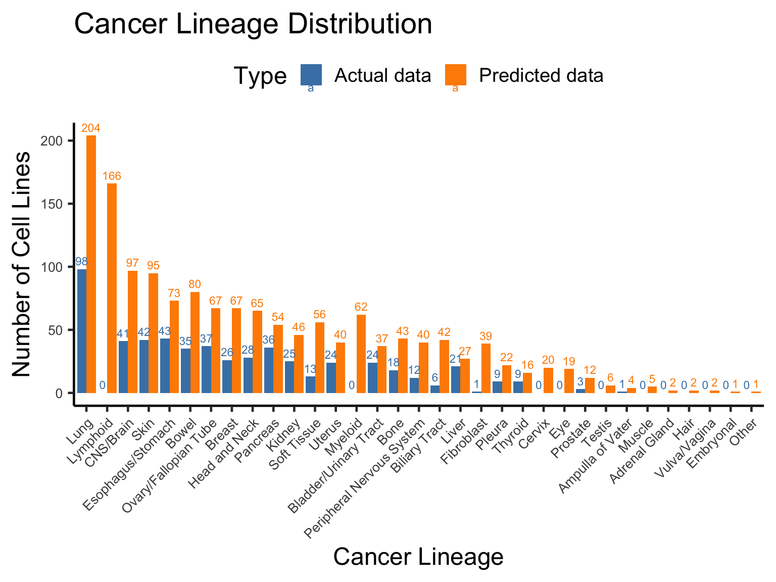
You can see here that the predicted data covers many more cancer lineages than the actual data, which may improve the power of downstream analyses.
Predicted Sensitivity by Lineage
Next, let’s see if the predicted Erlotinib LFC can better capture differences across cancer lineages.
# Plot actual vs predicted Erlotinib LFC boxplot faceted by LFC type and stratified by OncotreeLineage
plot_df <- erlotinib_compare_df |>
    select(Cell_Line, Actual_Erlotinib_LFC, Predicted_Erlotinib_LFC, OncotreeLineage) |>
    pivot_longer(
        cols = c(Actual_Erlotinib_LFC, Predicted_Erlotinib_LFC),
        names_to = "LFC_Type",
        values_to = "Erlotinib_LFC"
    ) |>
    na.omit()

lineage_counts <- plot_df |>
    group_by(OncotreeLineage) |>
    summarise(Count = n()) |>
    filter(Count >= 10)
plot_df <- plot_df |> filter(OncotreeLineage %in% lineage_counts$OncotreeLineage)

lineage_sort_by_predicted_LFC <- plot_df |>
    filter(LFC_Type == "Predicted_Erlotinib_LFC") |>
    group_by(OncotreeLineage) |>
    summarise(Median_Predicted_LFC = median(Erlotinib_LFC)) |>
    arrange(Median_Predicted_LFC) |>
    pull(OncotreeLineage)

plot_df$OncotreeLineage <- factor(plot_df$OncotreeLineage, levels = lineage_sort_by_predicted_LFC)

ggplot(plot_df, aes(x = OncotreeLineage, y = Erlotinib_LFC, color = LFC_Type)) +
    geom_jitter(width = 0.2, size = 2, alpha = 0.5) +
    geom_boxplot(outliers = FALSE, fill = "grey99", alpha = 0.3) +
    facet_wrap(~LFC_Type,
        nrow = 2, scales = "free_y",
        labeller = as_labeller(c(Actual_Erlotinib_LFC = "Actual Erlotinib LFC", Predicted_Erlotinib_LFC = "Predicted Erlotinib LFC"))
    ) +
    theme_classic(base_size = 18) +
    scale_color_manual(
        values = c(Actual_Erlotinib_LFC = "steelblue", Predicted_Erlotinib_LFC = "darkorange"),
        labels = c("Actual Erlotinib LFC", "Predicted Erlotinib LFC")
    ) +
    labs(
        title = "Erlotinib LFC by Cancer Lineage",
        x = "Cancer Lineage",
        y = "Erlotinib LFC"
    ) +
    geom_hline(yintercept = 0, linetype = "dashed", color = "grey30") +
    theme(
        axis.text.x = element_text(angle = 60, hjust = 1),
        legend.position = "none"
    )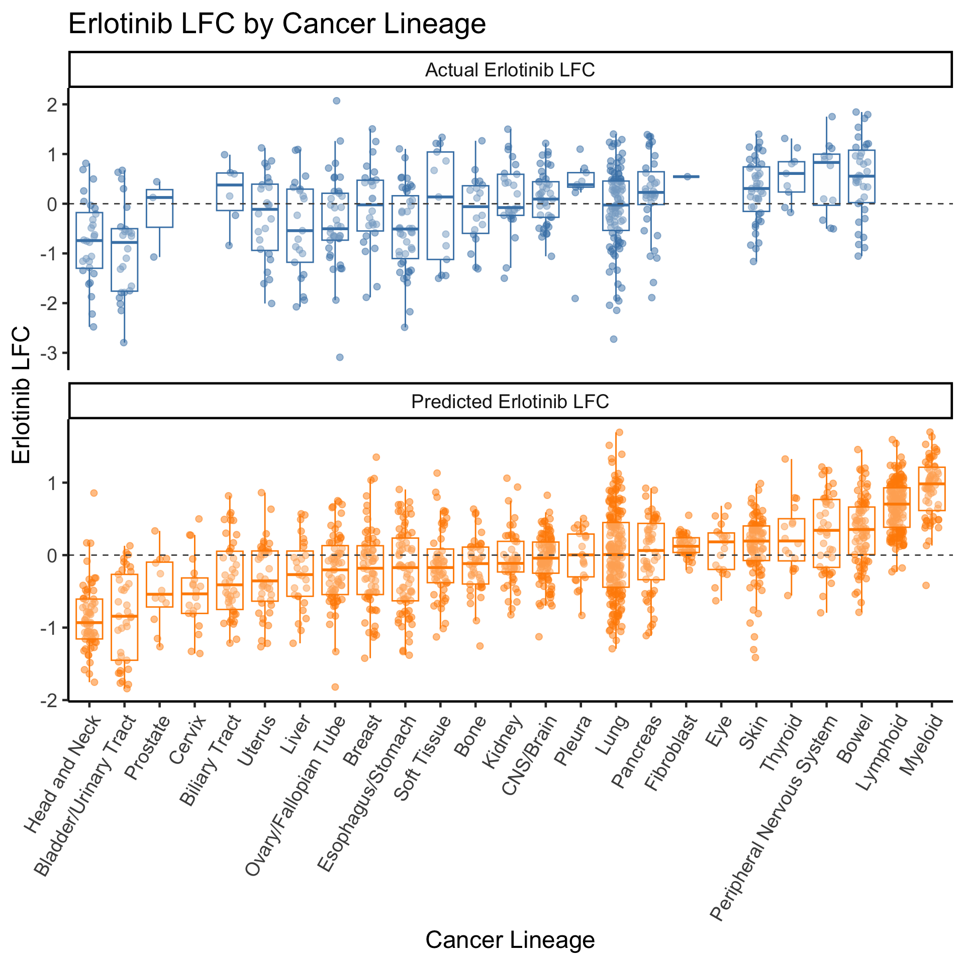
Result: Predicted data discovered lineage sensitivity for prostate, cervix, biliary tract; and showed that blood lineages are likely not sensitive.
Predicted Sensitivity by EGFR Mutation Status
Finally, let’s see whether the predicted Erlotinib LFC can capture known biological associations, such as sensitivity in EGFR mutant cell lines.
if (exists("egfr_mutation_status")) {
    # Compare predicted vs actual Erlotinib LFC between EGFR mutant and wildtype cell lines
    plot_df <- erlotinib_compare_df |>
        select(Cell_Line, Actual_Erlotinib_LFC, Predicted_Erlotinib_LFC, EGFR_Mutation_Status) |>
        pivot_longer(
            cols = c(Actual_Erlotinib_LFC, Predicted_Erlotinib_LFC),
            names_to = "LFC_Type",
            values_to = "Erlotinib_LFC"
        ) |>
        na.omit()

    # Plot boxplot: EGFR mutant vs wildtype facet by actual vs predicted with test p-value
    ggplot(plot_df, aes(x = EGFR_Mutation_Status, y = Erlotinib_LFC, color = EGFR_Mutation_Status)) +
        geom_boxplot(alpha = 1, outliers = FALSE) +
        geom_jitter(width = 0.2, size = 2, alpha = 0.5) +
        facet_wrap(~LFC_Type, nrow = 1, labeller = as_labeller(c(Actual_Erlotinib_LFC = "Actual Erlotinib LFC", Predicted_Erlotinib_LFC = "Predicted Erlotinib LFC"))) +
        theme_classic(base_size = 18) +
        labs(
            title = "Erlotinib LFC by EGFR Mutation Status",
            x = "EGFR Hotspot Mutation Status",
            y = "Erlotinib LFC"
        ) +
        scale_color_manual(values = c("Wildtype" = "darkgreen", "Heterozygous Mutant" = "darkorange", "Homozygous Mutant" = "darkred")) +
        theme(
            legend.position = "none",
            axis.text.x = element_text(angle = 45, hjust = 1)
        ) +
        stat_compare_means(aes(group = EGFR_Mutation_Status), label.y.npc = 0.9, size = 5)
} else {
    print("EGFR mutation data not loaded.")
}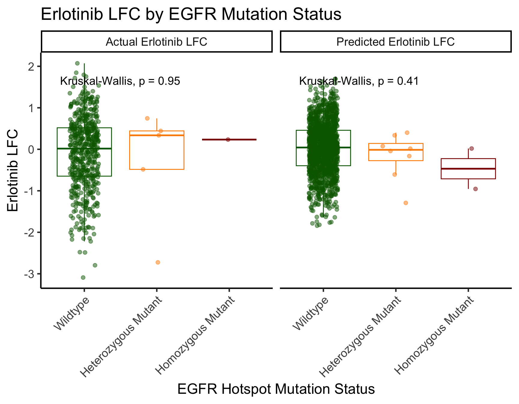
It seems that even in the predicted data, there is only a marginal difference in Erlotinib LFC between EGFR mutant and wildtype cell lines. This could be due to the fact that EGFR mutation instances are relatively rare in all of DepMap cell lines.
Summary
Here I demonstrated how to train an elastic net model using R’s Caret package with hyperparameter tuning via cross-validation from end to end. I showed the top 20 sensitivity and resistance predictor genes identified by the final model. I then applied the final model to all available DepMap cell lines to generate Erlotinib sensitivity predictions.
Finally, I showed that the predicted data can provide additional insights beyond the measured data, such as covering more cancer lineages. However, some known biological associations (e.g. EGFR mutation status) may still be difficult to capture due to data limitations.
Overall, this framework can be useful for generating drug sensitivity predictions for cell lines without measured data, which can aid in drug repurposing and precision oncology efforts.
References
- DepMap Portal: https://depmap.org/portal/
- Caret Package Documentation: https://topepo.github.io/caret/
- Applied Predictive Modeling by Kuhn and Johnson: https://www.springer.com/gp/book/9781461468486