import pandas as pd
import matplotlib.pyplot as plt
import numpy as np
import os

# Define file paths (relative to the ML_practice directory)
# Here I have preprocessed the data for this demo so the cell lines (rows) are aligned
sample_info_path = "ML_practice/sample_info.csv"
chronos_path = "ML_practice/chronos_dat.csv"
ge_path = "ML_practice/ccle_ge.csv"

# Load the datasets
# Sample metadata containing cell line information
sample_data = pd.read_csv(sample_info_path)

# Chronos scores: Gene effect scores from CRISPR knockout screens
chronos_dat = pd.read_csv(chronos_path)

# Gene Expression data: mRNA expression levels log2(TPM + 1)
ge_dat = pd.read_csv(ge_path)Training a Random Forest model with Scikit-Learn on DepMap data
Python
Machine Learning
DepMap
Random Forest
Scikit-Learn
Pandas
Introduction
In this specific blog post, we will explore the Cancer Dependency Map (DepMap) dataset to understand the relationship between genetic dependencies (CRISPR knockout effects) and gene expression levels. We will use Python’s pandas ecosystem for data loading, exploratory data analysis, and visualization. We will also use scikit-learn’s functions to build a Random Forest predictor pipeline that performs preprocessing, imputes missing values, and tunes hyperparameters. Finally, we will evaluate the model’s performance and extract genes that are most important for predicting gene dependency.
Data Loading
First, we import the necessary libraries and load the datasets. We are using three main datasets:
- Sample Info: Metadata about the cell lines (lineage, disease subtype, etc.).
- Chronos Data: CRISPR knockout scores representing gene dependency (lower score = higher dependency).
- Gene Expression (GE) Data: RNA-seq expression levels for various genes.
Data can be downloaded from here (modified from DepMap 24Q2): https://zenodo.org/records/17970100
Exploratory Data Analysis
Let’s inspect the structure and basic statistics of our datasets.
Sample Information
Checking the metadata to understand the cell lines we are working with.
# Display dataset information: columns, non-null counts, and data types
print("Sample Data Info:")
sample_data.info()
Sample Data Info:
<class 'pandas.core.frame.DataFrame'>
RangeIndex: 1959 entries, 0 to 1958
Data columns (total 9 columns):
# Column Non-Null Count Dtype
--- ------ -------------- -----
0 ModelID 1959 non-null object
1 StrippedCellLineName 1959 non-null object
2 CCLEName 1902 non-null object
3 OncotreeLineage 1954 non-null object
4 OncotreeSubtype 1959 non-null object
5 OncotreePrimaryDisease 1959 non-null object
6 LegacySubSubtype 831 non-null object
7 LegacyMolecularSubtype 151 non-null object
8 PatientMolecularSubtype 138 non-null object
dtypes: object(9)
memory usage: 137.9+ KBChronos (Dependency) Data
This dataset contains dependency scores for key genes like SMARCA2, SOX10, and KRAS.
# Display dataset information for Chronos data
print("\nChronos Data Info:")
chronos_dat.info()
Chronos Data Info:
<class 'pandas.core.frame.DataFrame'>
RangeIndex: 1959 entries, 0 to 1958
Data columns (total 4 columns):
 #   Column     Non-Null Count  Dtype
---  ------     --------------  -----
 0   cell_line  1959 non-null   object
 1   SMARCA2    1150 non-null   float64
 2   SOX10      1150 non-null   float64
 3   KRAS       1150 non-null   float64
dtypes: float64(3), object(1)
memory usage: 61.3+ KB
Gene Expression Data
This dataset provides expression levels for a wide range of genes across the cell lines.
# Display dataset information for Gene Expression data
print("\nGene Expression Data Info:")
ge_dat.info()
print("\nFirst 5 rows of Gene Expression Data:")
display(ge_dat.head())
Gene Expression Data Info:
<class 'pandas.core.frame.DataFrame'>
RangeIndex: 1959 entries, 0 to 1958
Columns: 19153 entries, TSPAN6 to CDR1
dtypes: float64(19153)
memory usage: 286.3 MB

First 5 rows of Gene Expression Data:| TSPAN6 | TNMD | DPM1 | SCYL3 | FIRRM | FGR | CFH | FUCA2 | GCLC | NFYA | ... | SPDYE11 | H3C2 | H3C3 | DUS4L-BCAP29 | C8orf44-SGK3 | ELOA3BP | NPBWR1 | ELOA3DP | ELOA3P | CDR1 | |
|---|---|---|---|---|---|---|---|---|---|---|---|---|---|---|---|---|---|---|---|---|---|
| 0 | 5.183487 | 0.000000 | 7.497612 | 2.107688 | 4.217231 | 0.042644 | 0.903038 | 5.722193 | 4.676944 | 3.720278 | ... | 0.056584 | 1.137504 | 0.000000 | 1.794936 | 0.201634 | 0.000000 | 0.028569 | 0.0 | 0.214125 | 0.014355 |
| 1 | 0.176323 | 0.000000 | 5.702103 | 1.238787 | 3.119356 | 4.141596 | 0.163499 | 4.134221 | 4.111866 | 2.347666 | ... | 0.000000 | 1.952334 | 0.238787 | 1.516015 | 0.000000 | 0.000000 | 0.028569 | 0.0 | 0.000000 | 0.000000 |
| 2 | 5.309976 | 0.084064 | 7.846117 | 1.875780 | 3.894333 | 0.000000 | 0.056584 | 6.666615 | 4.738768 | 3.984589 | ... | 0.014355 | 0.918386 | 0.000000 | 1.655352 | 0.000000 | 0.028569 | 0.000000 | 0.0 | 0.028569 | 0.000000 |
| 3 | 2.176323 | 0.000000 | 5.454505 | 2.480265 | 3.921246 | 0.887525 | 4.958843 | 3.949535 | 4.877253 | 4.829850 | ... | 0.014355 | 0.536053 | 0.505891 | 2.643856 | 0.097611 | 0.000000 | 0.000000 | 0.0 | 0.000000 | 0.000000 |
| 4 | 2.451541 | 0.000000 | 5.884842 | 2.927896 | 5.299391 | 0.201634 | 5.759156 | 4.150560 | 5.531069 | 5.029895 | ... | 0.000000 | 0.895303 | 1.350497 | 2.709291 | 0.678072 | 0.000000 | 0.000000 | 0.0 | 0.000000 | 0.000000 |
5 rows × 19153 columns
Data Distribution and Correlations
We can look at the overall distribution of the dependency data using a scatter matrix. This helps us spot potential correlations or clusters between different gene dependencies.
from pandas.plotting import scatter_matrix

# Create a scatter matrix to visualize pair-wise relationships in the Chronos dataset
# This includes histograms on the diagonal and scatter plots on off-diagonals
scatter_matrix(chronos_dat)
plt.show()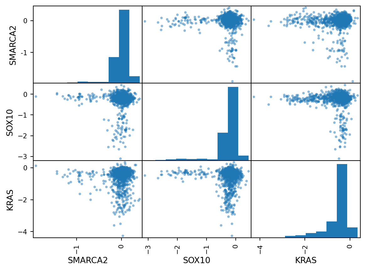
Let’s verify the correlations numerically. We drop the ‘cell_line’ column as it is categorical.
# Calculate the correlation matrix for the numeric columns in Chronos data
chronos_corr = chronos_dat.drop("cell_line", axis=1).corr()
print("\nCorrelation Matrix (Chronos Data):")
print(chronos_corr)
Correlation Matrix (Chronos Data):
          SMARCA2     SOX10      KRAS
SMARCA2  1.000000 -0.032416  0.005902
SOX10   -0.032416  1.000000 -0.052455
KRAS     0.005902 -0.052455  1.000000
Visualization: Dependency vs. Expression
A key question in cancer biology is whether gene expression predicts dependency. For example, if a cell line highly expresses SOX10, is it more dependent on SOX10 for survival (lower Chronos score)?
Let’s visualize the relationship between SOX10 dependency (Chronos score) and SOX10 gene expression.
# Plot SOX10 Chronos score (x-axis) vs SOX10 Gene Expression (y-axis)
# Note: Lower Chronos score means higher dependency.
plt.figure(figsize=(8, 6))
plt.scatter(chronos_dat["SOX10"], ge_dat["SOX10"], alpha=0.6)
plt.xlabel("SOX10 Chronos Score (Dependency)")
plt.ylabel("SOX10 Gene Expression")
plt.title("SOX10: Dependency vs Expression")
plt.grid(True, linestyle='--', alpha=0.5)
plt.show()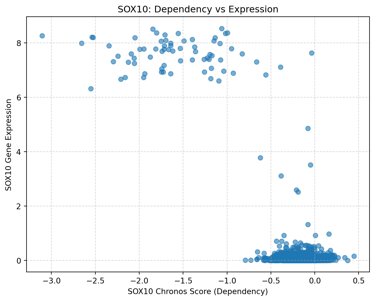
Finally, let’s calculate the Pearson correlation coefficient between these two variables to quantify the relationship.
# Calculate Pearson correlation between SOX10 dependency and expression
sox10_corr = chronos_dat["SOX10"].corr(ge_dat["SOX10"])
print(f"Pearson Correlation between SOX10 Chronos and Gene Expression: {sox10_corr:.4f}")
Pearson Correlation between SOX10 Chronos and Gene Expression: -0.8491This correlation value suggests a strong relationship between SOX10 gene expression and dependency.
Machine Learning
Now we will build a machine learning model to predict the SOX10 dependency score based on the gene expression profile of the cell lines.
Data Preprocessing
Before training, we need to prepare our data.
- Alignment: Ensure the cell lines in the dependency dataset match those in the gene expression dataset.
- Merging: Combined the target variable (SOX10 Chronos score) with the feature set (Gene Expression).
- Imputation: Dealing with missing values using K-Nearest Neighbors (KNN) imputation.
# Align and merge data
# The rows are already pre-aligned by cell line index
# Adding target variable to the dataframe for alignment
ge_dat = pd.read_csv(ge_path)
ge_dat["SOX10_chronos"] = chronos_dat["SOX10"]

# Remove rows where the target (SOX10_chronos) is NaN, as we can't train/test on them
ge_dat_clean = ge_dat.dropna(subset=["SOX10_chronos"])

# Separate features (X) and target (y)
X = ge_dat_clean.drop("SOX10_chronos", axis=1)
y = ge_dat_clean["SOX10_chronos"]

print(f"Data shape after removing missing targets: {X.shape}")
Data shape after removing missing targets: (1150, 19153)We will handle missing values in the features (Gene Expression) using KNN Imputation within our modeling pipeline.
Model Training
We will use a Random Forest Regressor to predict the dependency score.
Data Splitting
First, we split the data into training and testing sets (80% train, 20% test).
from sklearn.model_selection import train_test_split

# Split data into training and testing set
X_train, X_test, y_train, y_test = train_test_split(X, y, test_size=0.2, random_state=42)

print(f"Training samples: {X_train.shape[0]}")
print(f"Testing samples: {X_test.shape[0]}")
Training samples: 920
Testing samples: 230Pipeline and Hyperparameter Tuning
We create a pipeline that: 1. Imputes missing values using KNNImputer. 2. Scales features using StandardScaler (optional for RF but good practice). 3. Trains a RandomForestRegressor.
We will use RandomizedSearchCV to find the best hyperparameters (e.g., max_features for the Random Forest).
from sklearn.ensemble import RandomForestRegressor
from sklearn.model_selection import RandomizedSearchCV
from scipy.stats import randint
from sklearn.pipeline import Pipeline
from sklearn.preprocessing import StandardScaler
from sklearn.impute import KNNImputer

# Create a pipeline
pipeline = Pipeline([
    ("imputer", KNNImputer(n_neighbors=10)),
    ("scaler", StandardScaler()),
    ("rf", RandomForestRegressor(random_state=42))
])

# Define hyperparameter search space
param_dist = {
    'rf__max_features': randint(low=100, high=5000), # Number of features to consider at each split
    'rf__n_estimators': randint(low=50, high=200) # Number of trees in the forest
}

# Initialize RandomizedSearchCV
# n_iter=5 to keep run time reasonable for this demo
rnd_search = RandomizedSearchCV(
    pipeline,
    param_distributions=param_dist,
    n_iter=5, # Number of parameter settings that are sampled
    cv=3, # Number of folds in cross-validation
    random_state=42, # Random state for reproducibility
    scoring="neg_root_mean_squared_error", # Scoring metric
    n_jobs=-1 # Use all available CPU cores
)

# Fit the model
print("Training Random Forest model...")
rnd_search.fit(X_train, y_train)

print(f"Best RMSE: {-rnd_search.best_score_:.4f}")
print(f"Best Parameters: {rnd_search.best_params_}")

# Get the best model
final_model = rnd_search.best_estimator_
Training Random Forest model...Best RMSE: 0.2097
Best Parameters: {'rf__max_features': 3019, 'rf__n_estimators': 180}Model Evaluation
Now we evaluate the model’s performance on the unseen test set and investigate which genes are most important for predicting SOX10 dependency.
Feature Importance
Which genes’ expression levels are most predictive of SOX10 dependency?
# Extract feature importances
rf_model = final_model.named_steps['rf']
importances = rf_model.feature_importances_
feature_names = X.columns

# Create a dataframe for visualization
feat_importances = pd.Series(importances, index=feature_names)
top_features = feat_importances.nlargest(20)

# Plot top 20 features
plt.figure(figsize=(10, 6))
top_features.plot(kind='bar')
plt.title("Top 20 Feature Importances")
plt.ylabel("Importance")
plt.xlabel("Gene")
plt.xticks(rotation=45, ha='right')
plt.show()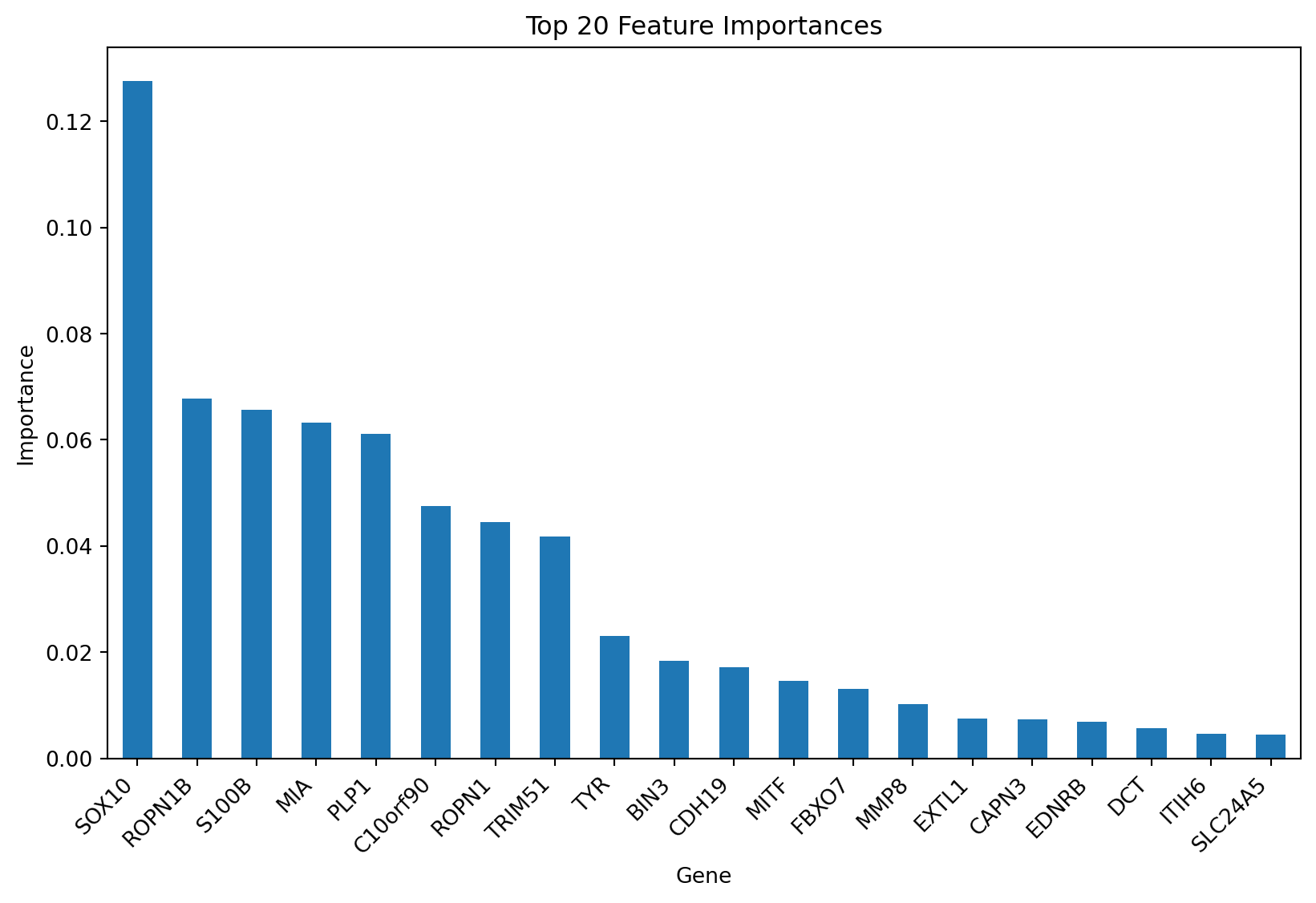
As expected, SOX10 gene expression is the most important feature for predicting SOX10 dependency.
Prediction Performance
We calculate the Root Mean Squared Error (RMSE) on the test set and visualize the predictions vs actual values.
from sklearn.metrics import mean_squared_error

# Predict on test set
test_predictions = final_model.predict(X_test)

# Calculate RMSE
test_mse = mean_squared_error(y_test, test_predictions)
test_rmse = np.sqrt(test_mse)

print(f"Test Set RMSE: {test_rmse:.4f}")

# Plot Predicted vs Expected
plt.figure(figsize=(8, 6))
plt.scatter(y_test, test_predictions, alpha=0.6)
plt.plot([y.min(), y.max()], [y.min(), y.max()], 'k--', lw=2) # Identity line
plt.xlabel("Expected Score (True)")
plt.ylabel("Predicted Score")
plt.title("Test Set: Predicted vs Expected")
plt.grid(True, linestyle='--', alpha=0.5)
plt.show()
Test Set RMSE: 0.2139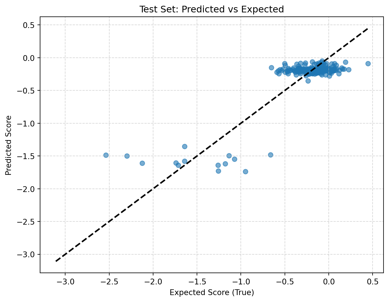
We can see that the model predicts a more bimodal distribution of scores than the actual data, although it does somewhat differentiate between high and low dependency populations. To improve the model, we could try to tune the hyperparameters further, or try different feature selection methods.